1 Introduction
This is the fifth part of a series where I work through the practice questions of the second edition of Richard McElreaths Statistical Rethinking.
Each post covers a new chapter and you can see the posts on previous chapters here.
You can find the the lectures and homework accompanying the book here.
The colours for this blog post are:
coral <- "#CD7672"
mint <- "#138086"
purple <- "#534666"
yellow <- "#EEb462"
The online version of the Statistical Rethinking, provided by the brilliant Erik Kusch, is missing a lot of practive questions, so I will focus on the examples from the print version here.
2 Easy practices
2.1 Question 6E1
List three mechanisms by which multiple regression can produce false inferences about causal effect.
The tree examples mentioned throughout the chapter were:
- Collinearity
- Post-treatment bias
- Collider bias
2.2 Question 6E2
For one of the mechanisms in the previous problem, provide an example of your choice, perhaps from your own research.
Collinearity
If you want to estimate the effect of geographic range on the extinction risk organism in the fossil record, you can choose between a range of potential parameters that express geographic range. For example, you can use the convex hull area or the maximum pairwise great circle distance. However, if you add both parameters in a model their true magnitude of association to extinction risk is lowered or even hidden, as they both encapsulate the same information.Post-treatment bias
Assume you want to estimate the effect of global mean temperature on the extinction risk of marine species in the fossil record. Additionally, you have an amazing data set on continental shelve area through time and would love to include that as well. However, temperature is quite likely causally related to shelve area as it drives eustatic sea level. So including shelve area in a model would shut the path between temperature and extinction risk, even though there is a real causal association.Collider bias
If anyone has a good example for a collider bias in palaeobiology, just message me on twitter (@GregorMathes).
2.3 Question 6E3
List the four elemental confounds. Can you explain the conditional dependencies of each?
- Pipe
dagitty("dag{
        X -> Y -> Z}") %>%
  impliedConditionalIndependencies()
## X _||_ Z | YIf we condition on Y, we shut the path between X and Z.
- Fork
dagitty("dag{
        X <- Y -> Z}") %>%
  impliedConditionalIndependencies()
## X _||_ Z | YIf we condition on Y, then learning X tells us nothing about Z. All the information is in Y.
- Collider
dagitty("dag{
        X -> Y <- Z}") %>%
  impliedConditionalIndependencies()
## X _||_ ZX is independent of Z. But conditioning on Y would open the path, and then X
would be dependent on Z conditional on Y.
- Descendant
dagitty("dag{
        X -> Y -> Z
        Y -> W}") %>%
  impliedConditionalIndependencies()
## W _||_ X | Y
## W _||_ Z | Y
## X _||_ Z | YThis is interesting. In the chapter, it says that if we would condition on W,
we would condition on Y as well (to a lesser extent). So I would have expected
X || Z | W here.
2.4 Question 6E4
How is a biased sample like conditioning on a collider? Think of the example at the open of the chapter.
Assume the collider X -> Y <- Z.Conditioning on a collider Y opens a path between X and Z, and leads to a spurious correlation between between these. This is similar to selection bias, where the researcher that sampled the data (or nature itself) cared about both X and Z when generating the sample.
3 Medium practices
3.1 Question 6M1
Modify the DAG on page 190 (page 186 in print) to include the variable V, an unobserved cause of C and Y: C <- V -> Y. Reanalyze the DAG. How many paths connect X to Y? Which must be closed? Which variables should you condition on now?
Let’s update the DAG using the ggdag package:
tribble(
  ~ name,  ~ x,  ~ y,
    "A",    1,     3,
    "U",    0,     2,
    "C",    2,     2,
    "V",    3,     1,
    "B",    1,     1,
    "X",    0,     0,
    "Y",    2,     0
) %>%
  dagify(
    Y ~ X + C + V,
         C ~ V + A,
         B ~ C + U,
         U ~ A,
         X ~ U,
         coords = .) %>%
  ggplot(aes(x = x, y = y, xend = xend, yend = yend)) +
  geom_dag_node(internal_colour = mint, alpha = 0.8, colour = "white") +
  geom_dag_text(aes(label = name), color = purple, size = 5) +
  geom_dag_edges(edge_color = purple) +
  labs(caption = "Figure 1: Adjusted DAG from the chapter, including V.") +
  theme_void()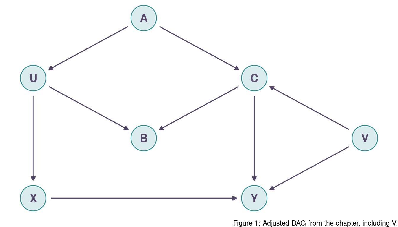
For the visual representations of the DAGs later on in this post, I will not show the code to generate the DAG plots to reduce the visual load on the reader. Anyways, you can look at the Rmd file with the raw code here.
So let’s first identify each path from X to Y.
(1) X -> Y
(2) X <- U <- A -> C -> Y
(3) X <- U <- A -> C <- V -> Y
(4) X <- U -> B <- C -> Y
(5) X <- U -> B <- C <- V -> Y
C is now a collider in path (3) and the path is closed. Additionally, both paths passing through B are closed as well as B stays a collider. The only open backdoor path is (2), and to close this path we can condition on A.
3.2 Question 6M2
Sometimes, in order to avoid multicollinearity, people inspect pairwise correlations among predictors before including them in a model. This is a bad procedure, because what matters is the conditional association, not the association before the variables are included in the model. To highlight this, consider the DAG X -> Z -> Y. Simulate data from this DAG so that the correlation between X and Z is very large. Then include both in a model prediction Y. Do you observe any multicollinearity? Why or why not? What is different from the legs example in the chapter?
The simulation is rather simple. We let Z be completely dependent on X with just a little bit of noise, and render Y then completely dependent on Z. Note that I standardize each value to choose the priors more easily.
sim_dat <- tibble(x = rnorm(1e4),
                  z = rnorm(1e4, x, 0.5),
                  y = rnorm(1e4, z)) %>%
  mutate(across(everything(), standardize))
The correlation between X and Z is hence really large as all information flows through this path.
sim_dat %>%
  summarise(correlation = cor(x, z))
## # A tibble: 1 x 1
## correlation
## <dbl>
## 1 0.895Now let’s fit a model using quadratic approximation and plot the coefficients:
alist(y ~ dnorm(mu, sigma),
      mu <- a + bx*x + bz*z,
      a ~ dnorm(0, 0.2),
      c(bx, bz) ~ dnorm(0, 0.5),
      sigma ~ dexp(1)) %>%
  quap(data = sim_dat) %>%
  precis() %>%
  as_tibble(rownames = "estimate") %>%
  filter(estimate %in% c("bx", "bz")) %>%
  rename(lower_pi = `5.5%`, upper_pi = `94.5%`) %>%
  ggplot() +
  geom_linerange(aes(xmin = lower_pi, xmax = upper_pi, y = estimate),
                 size = 1.5, colour = mint) +
  geom_point(aes(x = mean, y = estimate),
             shape = 21, colour = "grey20", stroke = 1,
             size = 5, fill = purple) +
  labs(y = NULL, x = "Estimate", caption = "Figure 2: Coefficient plot for simulated data with
       collinearity.") +
  theme_minimal()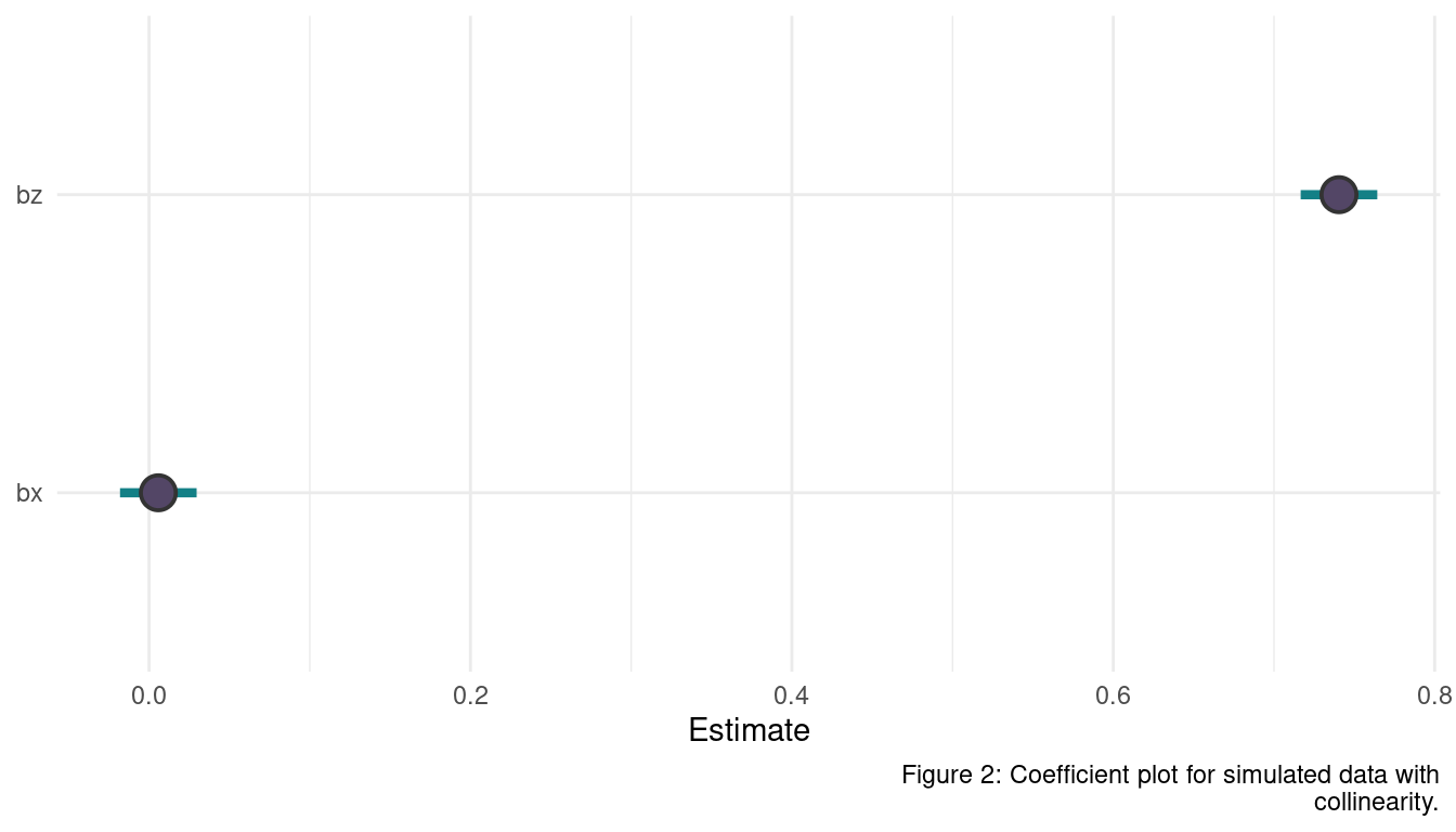
Not a big surprise, the effect of X is completely hidden as we condition on Z in a pipe. There is nothing new about X once the model knows Z. But to know that Z is only a mediatory variable, we need a causal model expressed in a DAG. The difference to the legs example here is that X and Z are causally related as X causes Z. It is therefore an example for a post-treatment bias. The leg lengths, on the other hand, where not causing each other, but were caused by a common parent instead:
leg1 <- Parent -> leg2
3.3 Question 6M3
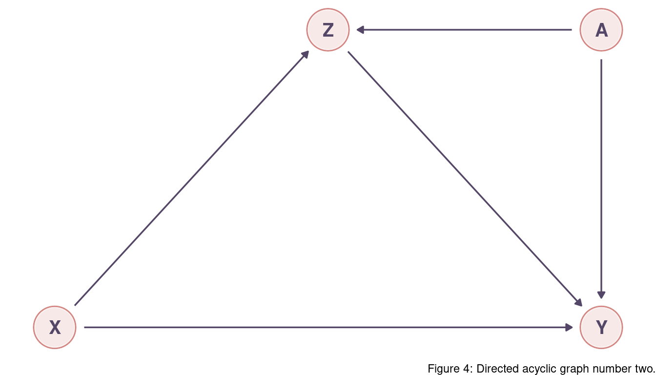
Learning to analyze DAGs requires practice. For each of the four DAGs below, state which variables, if any, you must adjust for (condition on) to estimate the total causal influence of X on Y.
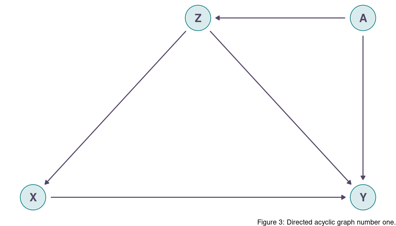
The are two backdoor paths, X <- Z -> Y and X <- Z <- A -> Y.
Both are open and go through Z, so we can simply condition on Z.
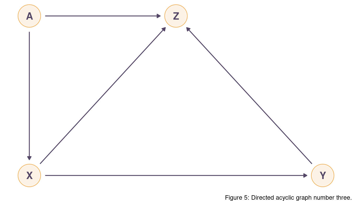
There are two backdoor paths, X -> Z -> Y and X -> Z <- A -> Y.
We want to keep X -> Z -> Y as it encapsulates information flowing from X to Y (and we
want to capture the total causal influence).
The second path is closed as Z is a collider here.
We don’t need to adjust for anything.
But note that conditioning on Z would open the second path and would be a mistake as it would create association between X on A.
There are two backdoor paths: X <- A -> Z <- Y and X -> Z <- Y.
Both paths are closed as Z is a collider for both.
We don’t need to condition on anything.
Again, inluding Z in a model would create spurios relationships that we want to avoid.
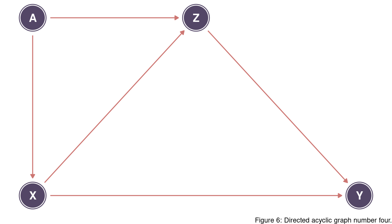
There are two backdoor paths: X <- A -> Z -> Y and X -> Z -> Y.
We want to keep the second one but close the first one. For this, we can condition on A. Conditioning on Z would close the first path as well, but also the second one which we want to keep as true causal.
4 Hard practices
4.1 Question 6H1
Use the Waffle House data, data(WaffleDivorce), to find the total causal influence of number of Waffle Houses on divorce rate. Justify your model or models with a causal graph.
Let’s load the data, standardise predictor and outcome and assign better names. We further transform south to an index variable: 1 is coded as not belonging to south, and 2 as belonging to south.
data("WaffleDivorce")

dat_waffle <- WaffleDivorce %>%
  as_tibble() %>%
  select(divorce = Divorce, age = MedianAgeMarriage,
         m_rate = Marriage, waffle = WaffleHouses,
         south = South) %>%
  mutate(across(-south, standardize),
         south = south + 1)
I assume that age (medium age at marriage) influence both divorce (divorce rate) and m_rate (marriage rate). This is something we could see in previous chapter. I further expect that south (southerness) influences both age and waffle (number of Waffle Houses).
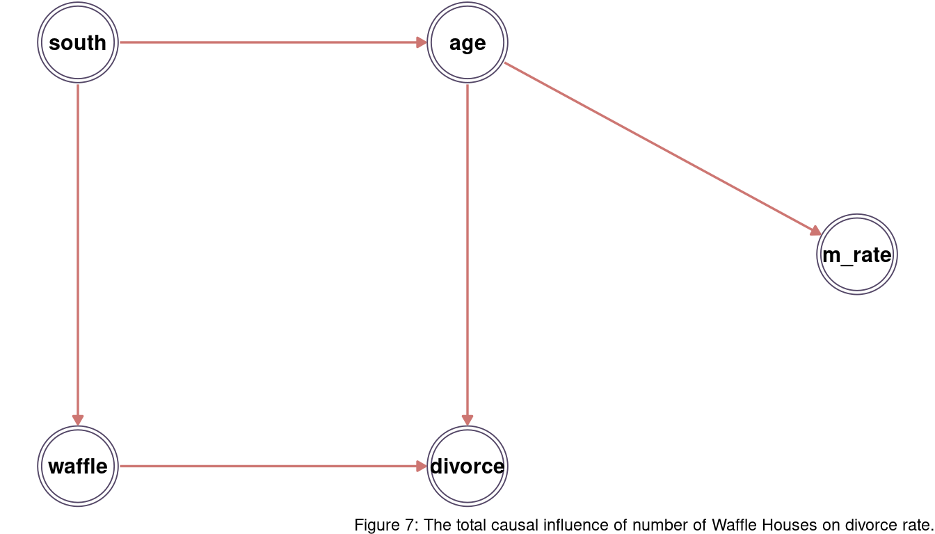
We can see that there is one open backdoor path from waffle <- south -> age -> divorce. We can close this path by conditioning on south.
m_waffle <- alist(
  divorce ~ dnorm(mu, sigma),
  mu <- a[south] + Bwaffle*waffle,
  a[south] ~ dnorm(0, 0.5),
  Bwaffle ~ dnorm(0, 0.5),
  sigma ~ dexp(1)) %>%
  quap(data = dat_waffle)
We can see that there is no information in waffle about divorce, that is not already in south.
m_waffle %>%
  precis() %>%
  as_tibble(rownames = "estimate") %>%
  filter(estimate == "Bwaffle") %>%
  mutate(across(where(is.numeric), round, digits = 2)) %>%
knitr::kable()| estimate | mean | sd | 5.5% | 94.5% |
|---|---|---|---|---|
| Bwaffle | 0.08 | 0.16 | -0.17 | 0.34 |
As we will look at coefficient estimates quite often in the hard practices, I will wrap up the code above into a helper function.
test_independence <- function(model.input, coeff.input, depth.output = 1){
  suppressWarnings(
    precis(model.input, depth = depth.output) %>%
    as_tibble(rownames = "estimate") %>%
    filter(estimate %in% {{coeff.input}}) %>%
    mutate(across(where(is.numeric), round, digits = 2)) %>%
    knitr::kable()
  )
}
We can visualise the association as well:
s <- seq(from = -2, to = 2, length.out = 30)
N <- 1e3

m_waffle %>%
  link(data = list(waffle = s,
                   south = 1)) %>%
  as_tibble() %>%
  pivot_longer(cols = everything(), values_to = "pred_divorce") %>%
  add_column(waffle = rep(s, N)) %>%
  group_by(waffle) %>%
  nest() %>%
  mutate(pred_divorce = map(data, "pred_divorce"),
         mean_divorce = map_dbl(pred_divorce, mean),
         pi = map(pred_divorce, PI),
         lower_pi = map_dbl(pi, pluck(1)),
         upper_pi = map_dbl(pi, pluck(2))) %>%
  select(waffle, mean_divorce, lower_pi, upper_pi) %>%
  ggplot() +
  geom_ribbon(aes(waffle, ymin = lower_pi, ymax = upper_pi),
              fill = mint, alpha = 0.3) +
  geom_line(aes(waffle, mean_divorce),
            size = 1.5, colour = coral) +
  coord_cartesian(ylim = c(-2, 2)) +
  labs(x = "Waffle (std)", y = "Divorce (std)",
       caption = "Figure 8: Total causal effect of number of Waffle House on Divorce,
       while keeping 'South' constant.") +
  theme_minimal()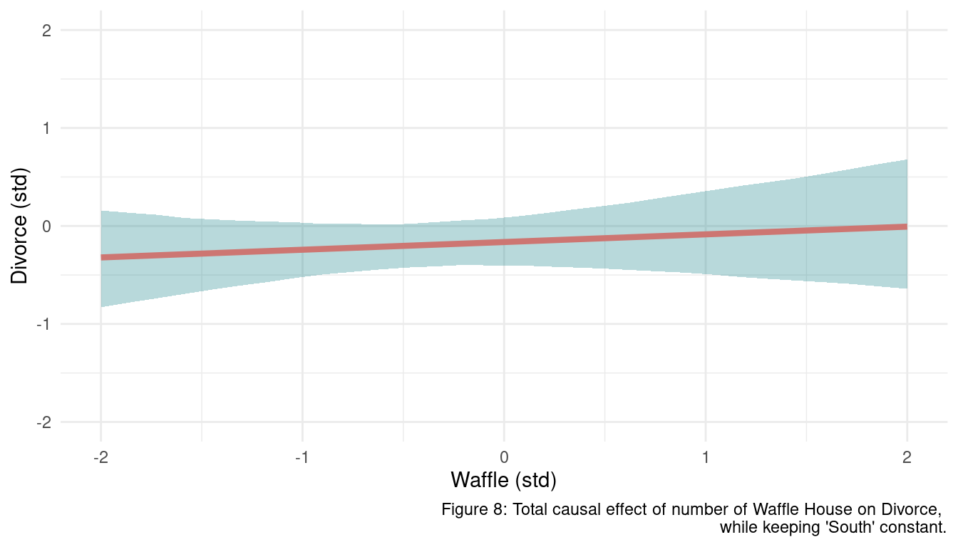
4.2 Question 6H2
Build a series of models to test the implied conditional independencies of the causal graph you used in the previous problem. If any of the tests fail, how do you think the graph needs to be amended? Does the graph need more or fewer arrows? Feel free to nominate variables that are not in the data.
Let’s first check the implied conditional independencies.
dagitty("dag{
        waffle -> divorce <- age <- south -> waffle
        age -> m_rate}") %>%
  impliedConditionalIndependencies()
## age _||_ wffl | soth
## dvrc _||_ m_rt | age
## dvrc _||_ soth | age, wffl
## m_rt _||_ soth | age
## m_rt _||_ wffl | soth
## m_rt _||_ wffl | ageLet’s start with age || waffle | south
alist(
  waffle ~ dnorm(mu, sigma),
  mu <- a[south] + Bage*age,
  a[south] ~ dnorm(0, 0.5),
  c(Bage) ~ dnorm(0, 0.5),
  sigma ~ dexp(1)) %>%
  quap(data = dat_waffle) %>%
test_independence(coeff.input = "Bage")| estimate | mean | sd | 5.5% | 94.5% |
|---|---|---|---|---|
| Bage | 0.03 | 0.1 | -0.13 | 0.2 |
age is independent of waffle after conditioning on south, as the posterior Bage shows no consistent association with waffle.
divorce || m_rate | age
alist(
  m_rate ~ dnorm(mu, sigma),
  mu <- a + Bdivorce*divorce + Bage*age,
  a ~ dnorm(0, 0.2),
  c(Bdivorce, Bage) ~ dnorm(0, 0.5),
  sigma ~ dexp(1)) %>%
  quap(data = dat_waffle) %>%
test_independence(coeff.input = "Bdivorce") | estimate | mean | sd | 5.5% | 94.5% |
|---|---|---|---|---|
| Bdivorce | -0.06 | 0.12 | -0.25 | 0.13 |
divorce is independent from m_rate after conditioning on age.
divorce || south | age, waffle
alist(
  divorce ~ dnorm(mu, sigma),
  mu <- a[south] + Bage*age + Bwaffle*waffle,
  a[south] ~ dnorm(0, 0.5),
  c(Bage, Bwaffle) ~ dnorm(0, 0.5),
  sigma ~ dexp(1)) %>%
  quap(data = dat_waffle) %>%
test_independence(depth.output = 2, coeff.input = c("a[1]", "a[2]"))| estimate | mean | sd | 5.5% | 94.5% |
|---|---|---|---|---|
| a[1] | -0.08 | 0.14 | -0.30 | 0.13 |
| a[2] | 0.20 | 0.23 | -0.17 | 0.57 |
south is independent from divorce after conditioning on age and waffle.
m_rate || south | age
alist(
  m_rate ~ dnorm(mu, sigma),
  mu <- a[south] + Bage*age,
  a[south] ~ dnorm(0, 0.5),
  Bage ~ dnorm(0, 0.5),
  sigma ~ dexp(1)) %>%
  quap(data = dat_waffle) %>%
test_independence(depth.output = 2, coeff.input = c("a[1]", "a[2]"))| estimate | mean | sd | 5.5% | 94.5% |
|---|---|---|---|---|
| a[1] | 0.06 | 0.11 | -0.12 | 0.23 |
| a[2] | -0.13 | 0.17 | -0.41 | 0.14 |
south is independent from m_rate after conditioning on age.
m_rate || waffle | south
alist(
  waffle ~ dnorm(mu, sigma),
  mu <- a[south] + Bm_rate*m_rate,
  a[south] ~ dnorm(0, 0.5),
  Bm_rate ~ dnorm(0, 0.5),
  sigma ~ dexp(1)) %>%
  quap(data = dat_waffle) %>%
test_independence(coeff.input = "Bm_rate")| estimate | mean | sd | 5.5% | 94.5% |
|---|---|---|---|---|
| Bm_rate | -0.02 | 0.1 | -0.18 | 0.14 |
m_rate is independent from waffle after conditioning on south.
m_rate || waffle | age
alist(
  waffle ~ dnorm(mu, sigma),
  mu <- a + Bm_rate*m_rate + Bage*age,
  a ~ dnorm(0, 0.2),
  c(Bm_rate, Bage) ~ dnorm(0, 0.5),
  sigma ~ dexp(1)) %>%
  quap(data = dat_waffle) %>%
test_independence(coeff.input = "Bm_rate")| estimate | mean | sd | 5.5% | 94.5% |
|---|---|---|---|---|
| Bm_rate | -0.09 | 0.18 | -0.38 | 0.2 |
m_rate is independent from waffle after conditioning on age.
4.3 Data foxes
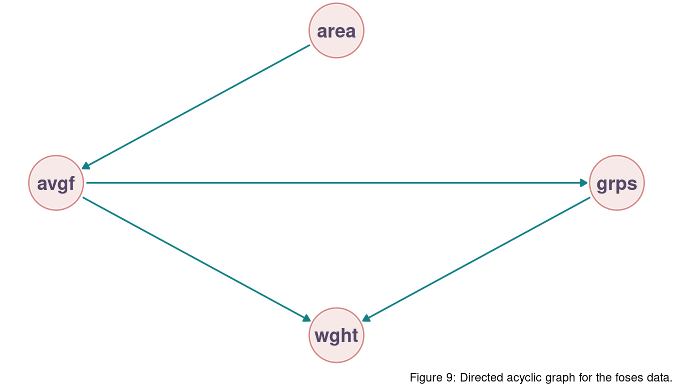
All three problems below are based on the same data. The data in data(foxes) are 116 foxes from 30 different urban groups in England. These foxes are like street gangs. Group size varies from 2 to 8 individuals. Each group maintains its own (almost exclusive) urban territory. Some territories are larger than others. The area variable encodes this information. Some territories also have more avgfood than others. We want to model the weight of each fox. For the problems below, assume this DAG:
4.4 Question 6H3
Use a model to infer the total causal influence of area on weight . Would increasing the area available to each fox make it heavier (healthier)? You might want to standardize the variables. Regardless, use prior predictive simulation to show that your model’s prior predictions stay within the possible outcome range.
There are two paths from area to weight:
(1) area -> avgfood -> weight
(2) area -> avgfood -> groupsize -> weight
Both of these paths are causal and we want to have them in our model. Note that we don’t have any backdoor paths and hence a simple linear regression with a single predictor is sufficient.
Let’s start by loading the data and standardizing all variables but group, which is a dummy variable.
data("foxes")

dat_foxes <- foxes %>%
  as_tibble() %>%
  mutate(across(-group, standardize))
Now we are ready to call the model.
m_foxes1 <- alist(weight ~ dnorm(mu, sigma),
                  mu <- a + Barea*area,
                  a ~ dnorm(0, 0.2),
                  Barea ~ dnorm(0, 0.5),
                  sigma ~ dexp(1)) %>%
  quap(data = dat_foxes)
Using prior predictive simulation as discussed in previous chapters, we can check if our priors are falling outside a realistic range.
m_foxes1 %>%
  extract.prior() %>%
  link(m_foxes1, post = .,
    data = list(area = seq(-2, 2, length.out = 20))) %>%
  as_tibble() %>%
  pivot_longer(cols = everything(), values_to = "weight") %>%
  add_column(
    area = rep(seq(-2, 2, length.out = 20), 1000),
    type = rep(as.character(1:1000), each = 20)) %>%
  ggplot() +
  geom_line(aes(x = area, y = weight, group = type),
            alpha = 0.1, colour = coral) +
  labs(x = "Area (std)", y = "Weight (std)",
       caption = "Figure 9: Prior predictive simulation for standardised area on weight.") +
  theme_minimal()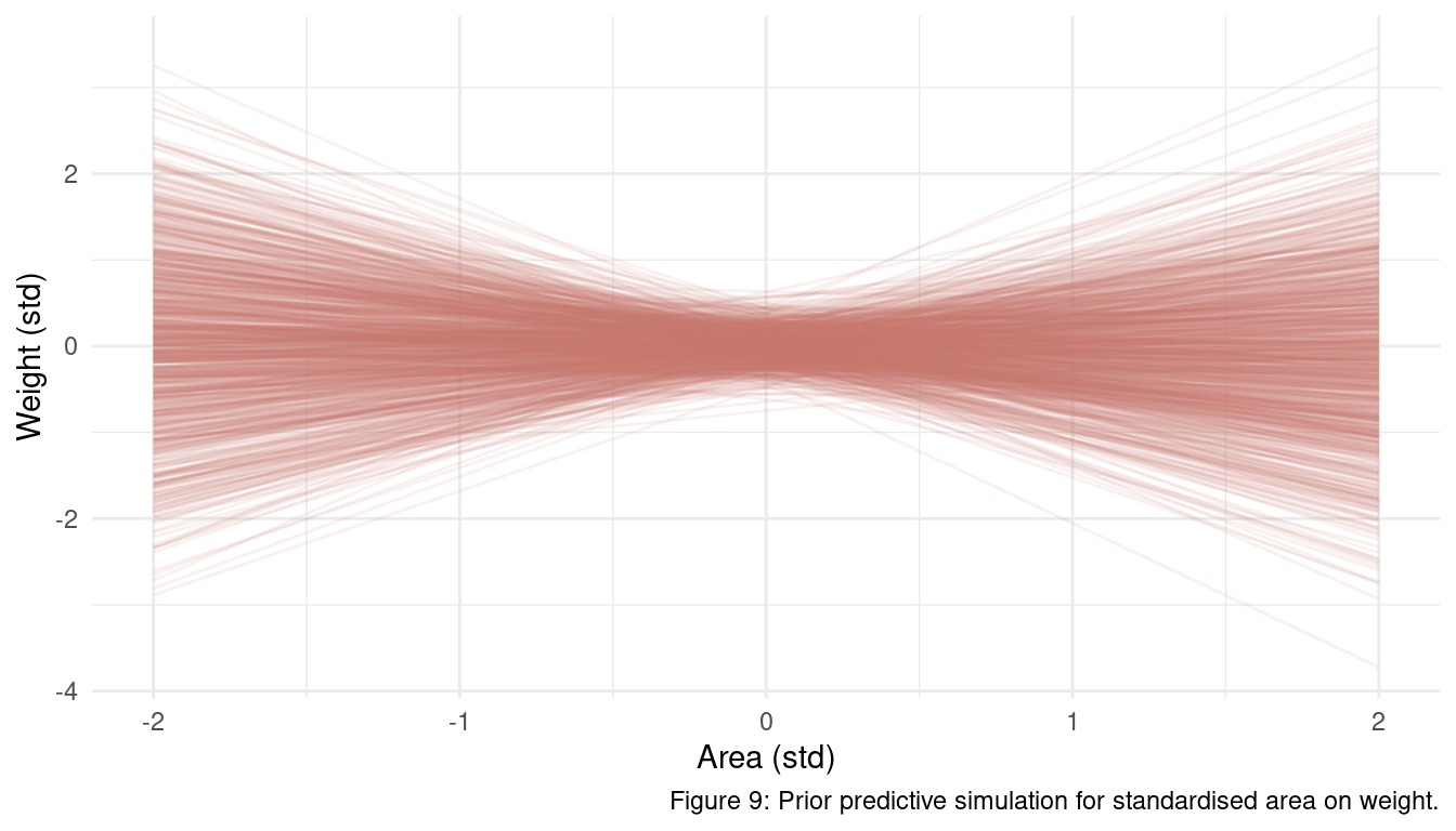
It almost seems like some of these lines are too extreme (outside of |-2, 2| sd) but they are still realistic. Anyone with some kind of knowledge about fox ecology can produce better priors than I am using here, but as I am really lazy I will stick to these rather uninformative priors for now.
Let’s see the effect of area on weight.
m_foxes1 %>%
test_independence(coeff.input = "Barea")| estimate | mean | sd | 5.5% | 94.5% |
|---|---|---|---|---|
| Barea | 0.02 | 0.09 | -0.13 | 0.16 |
There is no substantial association between area and weight.
4.5 Question 6H4
Now infer the causal impact of adding food (avgfood) to a territory. Would this make foxes heavier? Which covariates do you need to adjust for to estimate the total causal influence of food?
There are again two paths:
(1) avgfood -> groupsize -> weight
(2) avgfood -> weight
Both are open and we want to keep both to get the total causal impact of food on weight. Including groupsize (condition on groupsize) would close the first path, which we don’t want. Again, we don’t have any backdoor paths and a single predictor is enough.
alist(weight ~ dnorm(mu, sigma),
                  mu <- a + Bavgf*avgfood,
                  a ~ dnorm(0, 0.2),
                  Bavgf ~ dnorm(0, 0.5),
                  sigma ~ dexp(1)) %>%
  quap(data = dat_foxes) %>%
test_independence(coeff.input = "Bavgf")| estimate | mean | sd | 5.5% | 94.5% |
|---|---|---|---|---|
| Bavgf | -0.02 | 0.09 | -0.17 | 0.12 |
There is no substantial relationship between avgfood and weight. This is no big surprise as avgfood is only causally related to area (at least in our DAG), and area showed no dependency as well.
4.6 Question 6H5
Now infer the causal impact of group size. Which covariates do you need to adjust for? Looking at the posterior distribution of the resulting model, what do you think explains these data? That is, can you explain the estimates for all three problems? How do they make sense together?
We have two paths:
(1) groupsize -> weight
(2) groupsize -> avgfood -> weight
The second is a backdoor path and we want to close it (note that avgfood is a fork). We can do this by simply adjusting for avgfood.
alist(weight ~ dnorm(mu, sigma),
                  mu <- a + Bavgf*avgfood + Bgrps*groupsize,
                  a ~ dnorm(0, 0.2),
                  c(Bavgf, Bgrps) ~ dnorm(0, 0.5),
                  sigma ~ dexp(1)) %>%
  quap(data = dat_foxes) %>%
test_independence(coeff.input = c("Bavgf","Bgrps"))| estimate | mean | sd | 5.5% | 94.5% |
|---|---|---|---|---|
| Bavgf | 0.48 | 0.18 | 0.19 | 0.76 |
| Bgrps | -0.57 | 0.18 | -0.86 | -0.29 |
We can see that groupsize is negatively related to weight, and when groupsize is in the model the effect of avgfood on weight is positive. This looks like a masked relationship as the total causal effect of avgfood on weight was not substantial. It makes sense that foxes with more food are heavier, but more food means also that other foxes are attracted (or born) into the area. Now you have to distribute the food between more foxes, which cancels out the effect of avgfood on weight. More foxes means also that an individual fox has less food and therefore weighs less, leading to the negative relationship between groupsize and weight.
4.7 Question 6H6 and 6H7
Questions 6H6 and 6H7 are open research questions and I will hopefully manage to play around with them, once I have more time. So stick around for some updates of this post in the future.
5 Summary
I have read The book of why by Juda Pearl two years ago and thought to myself that this nicely plays out the route analysis in Palaeobiology (or in Science overall) should go. However, there was no way I could implement the statements from The book of why in my own research. There was no guide to go from theory to practice and I was lacking the tools. Turns out that this chapter in Statistical rethinking is providing the tools and the basics for causal inference. And this just makes me happy.
sessionInfo()## R version 4.0.3 (2020-10-10)
## Platform: x86_64-pc-linux-gnu (64-bit)
## Running under: Linux Mint 20.1
##
## Matrix products: default
## BLAS: /usr/lib/x86_64-linux-gnu/blas/libblas.so.3.9.0
## LAPACK: /usr/lib/x86_64-linux-gnu/lapack/liblapack.so.3.9.0
##
## locale:
## [1] LC_CTYPE=de_DE.UTF-8 LC_NUMERIC=C
## [3] LC_TIME=de_DE.UTF-8 LC_COLLATE=de_DE.UTF-8
## [5] LC_MONETARY=de_DE.UTF-8 LC_MESSAGES=de_DE.UTF-8
## [7] LC_PAPER=de_DE.UTF-8 LC_NAME=C
## [9] LC_ADDRESS=C LC_TELEPHONE=C
## [11] LC_MEASUREMENT=de_DE.UTF-8 LC_IDENTIFICATION=C
##
## attached base packages:
## [1] parallel stats graphics grDevices utils datasets methods
## [8] base
##
## other attached packages:
## [1] dagitty_0.3-1 ggdag_0.2.3 rethinking_2.13
## [4] rstan_2.21.2 StanHeaders_2.21.0-7 forcats_0.5.0
## [7] stringr_1.4.0 dplyr_1.0.3 purrr_0.3.4
## [10] readr_1.4.0 tidyr_1.1.2 tibble_3.0.5
## [13] ggplot2_3.3.3 tidyverse_1.3.0
##
## loaded via a namespace (and not attached):
## [1] matrixStats_0.57.0 fs_1.5.0 lubridate_1.7.9.2 httr_1.4.2
## [5] tools_4.0.3 backports_1.2.1 utf8_1.1.4 R6_2.5.0
## [9] DBI_1.1.1 colorspace_2.0-0 withr_2.4.1 tidyselect_1.1.0
## [13] gridExtra_2.3 prettyunits_1.1.1 processx_3.4.5 curl_4.3
## [17] compiler_4.0.3 cli_2.2.0 rvest_0.3.6 xml2_1.3.2
## [21] labeling_0.4.2 bookdown_0.21 scales_1.1.1 mvtnorm_1.1-1
## [25] callr_3.5.1 digest_0.6.27 rmarkdown_2.6 pkgconfig_2.0.3
## [29] htmltools_0.5.1.1 highr_0.8 dbplyr_2.0.0 rlang_0.4.10
## [33] readxl_1.3.1 rstudioapi_0.13 shape_1.4.5 generics_0.1.0
## [37] farver_2.0.3 jsonlite_1.7.2 inline_0.3.17 magrittr_2.0.1
## [41] loo_2.4.1 Rcpp_1.0.6 munsell_0.5.0 fansi_0.4.2
## [45] viridis_0.5.1 lifecycle_0.2.0 stringi_1.5.3 yaml_2.2.1
## [49] ggraph_2.0.4 MASS_7.3-53 pkgbuild_1.2.0 grid_4.0.3
## [53] ggrepel_0.9.1 crayon_1.3.4 lattice_0.20-41 graphlayouts_0.7.1
## [57] haven_2.3.1 hms_1.0.0 knitr_1.30 ps_1.5.0
## [61] pillar_1.4.7 igraph_1.2.6 boot_1.3-25 codetools_0.2-18
## [65] stats4_4.0.3 reprex_1.0.0 glue_1.4.2 evaluate_0.14
## [69] blogdown_1.1 V8_3.4.0 RcppParallel_5.0.2 modelr_0.1.8
## [73] tweenr_1.0.1 vctrs_0.3.6 cellranger_1.1.0 polyclip_1.10-0
## [77] gtable_0.3.0 assertthat_0.2.1 ggforce_0.3.2 xfun_0.20
## [81] broom_0.7.3 tidygraph_1.2.0 coda_0.19-4 viridisLite_0.3.0
## [85] ellipsis_0.3.1