1 Introduction
This is the sixth part of a series where I work through the practice questions of the second edition of Richard McElreaths Statistical Rethinking.
Each post covers a new chapter and you can see the posts on previous chapters here.
You can find the the lectures and homework accompanying the book here.
The colours for this blog post are:
red <- "#A4243B"
yellow <- "#D8973C"
brown <- "#BD632F"
grey <- "#273E47"
The homework for this week is the same as the hard practices.
2 Easy practices
2.1 Question 7E1
State the three motivating criteria that define information entropy. Try to express each in your own words.
- The measure of uncertainty should be continuous. Continuity enables the comparison of two measures.
- The measure of uncertainty should increase as the number of possible events in-creases. More events mean more uncertainty about which event will occur.
- The measure of uncertainty should be additive. We need to be able to add up all measures.
2.2 Question 7E2
Suppose a coin is weighted such that, when it is tossed and lands on a table, it comes up heads 70 % of the time. What is the entropy of this coin?
There are two events: 70 % heads and 30 % tails. Entropy is defined as \[H(p)=−\sum_{i=1}^n p_ilog(p_i) = −(p_Hlog(p_H)+p_Tlog(p_T))\]
We can transform this into R code:
inf_entropy <- function(p){
  -sum(p*log(p))
}
The function takes a vector as input and returns the entropy.
c(0.7, 0.3) %>%
  inf_entropy()
## [1] 0.6108643The entropy is 0.61.
2.3 Question 7E3
Suppose a four-sided die is loaded such that, when tossed onto a table, it shows “1” 20%, “2” 25%, ”3” 25%, and ”4” 30% of the time. What is the entropy of this die?
The defined function makes this quite easy:
c(0.2, 0.25, 0.25, 0.30) %>%
  inf_entropy()
## [1] 1.3762272.4 Question 7E4
Suppose another four-sided die is loaded such that it never shows “4”. The other three sides show equally often. What is the entropy of this die.
An event not occurring can be simply omitted. All other events have a probability of 1/3.
rep(1/3, 3) %>%
  inf_entropy()
## [1] 1.0986123 Medium practices
3.1 Question 7M1
Write down and compare the definitions of AIC and WAIC. Which of these criteria is most general? Which assumptions are required to transform the more general criterion into a less general one?
\[AIC = D_{train} + 2p = 2lppd + 2p\] where \(D_{train} =\) in-sample deviance and \(p =\) the number of free parameters in the posterior distribution.
The AIC is only reliable when:
(1) The priors are flat or overwhelmed by the likelihood.
(2) The posterior distribution is approximately multivariate Gaussian.
(3) The sample size N is much greater than the number of parameters k.
\[WAIC = −2(lppd −\sum_i(var_θ log p(y_i|θ))\]
where \(y_i =\) observation at point \(i\), \(θ =\) the posterior distribution,
\(lppd =\) log-pointwise-predictive density.
The WAIC is only reliable when:
(1) The sample size N is much greater than the number of parameters k.
Hence, the WAIC is similar to the AIC when the priors are flat or overwhelmed by the likelihood, and when the posterior distribution is approximately multivariate gaussian.
3.2 Question 7M2
Explain the difference between model selection and model comparison. What information is lost under model selection.
Model selection is the practice of choosing the model with the lowest criterion value and then discarding the others. Model comparison, on the other hand, uses uses multiple models to understand both how different variables influence predictions and, in combination with a causal model, implied conditional indendencies among variables help us infer causal relationships. With model selection, we are throwing away the differences in the information criterions between each model which encapsulates how confident we are in a model.
3.3 Question 7M3
When comparing models with an information criterion, why must all models be fit to exactly the same observations? What would happen to the information criterion values, if the models were fit to different numbers of observations? Perform some experiments, if you are not sure.
As information criterion is based on the deviance, which is a sum. More observations generally lead to a higher deviance as more values are summed up, rendering a comparison to a model with less observations useless. We can show this using a simulation approach
Let’s define a function that simulates data with N observations, runs a linear regression and returns the WAIC estimate:
waic_sim <- function(N){
  dat <- tibble(x = rnorm(N),
                y = rnorm(N)) %>%
    mutate(across(everything(), standardize))

  alist(
    x ~ dnorm(mu, 1),
    mu <- a + By*y,
    a ~ dnorm(0, 0.2),
    By ~ dnorm(0, 0.5)
  ) %>%
    quap(data = dat) %>%
    WAIC() %>%
    as_tibble() %>%
    pull(WAIC)
}
Now we define a sequence of N ranging from 100 to 1000 observations, apply the waic_sim function to each, save the results in a data frame and plot it.
seq(100, 1000, by = 100) %>%
  map_dbl(waic_sim) %>%
  enframe(name = "n_obs", value = "WAIC") %>%
  mutate(n_obs = seq(100, 1000, by = 100)) %>%
  ggplot(aes(n_obs, WAIC)) +
  geom_line(colour = grey) +
  geom_point(shape = 21, fill = red,
             colour = grey, size = 2.5,
             stroke = 1, alpha = 0.9) +
  labs(x = "Number of observations",
       caption = "Figure 1: Simulation of WAIC values of the same data
       based on the number of observations.") +
  theme_minimal()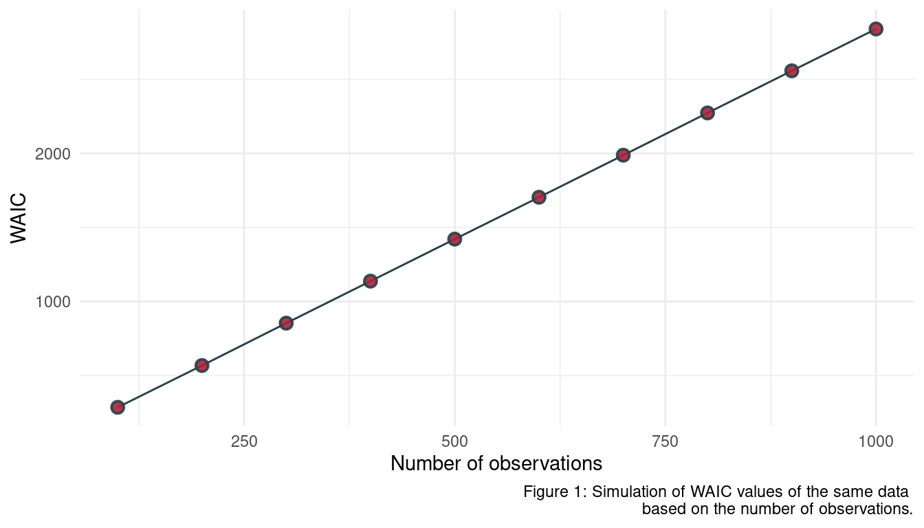
3.4 Question 7M4
What happens to the effective number of parameters, as measured by PSIS or WAIC, as a prior becomes more concentrated? Why? Perform some experiments, if you are not sure.
Experiments are always good, so let’s start. Similar to the approach above, we first define a function returning the estimate we want, in this case the number of parameters. But this time, the function takes a prior as an argument.
psis_sim <- function(prior){
  dat <- tibble(x = rnorm(10),
                y = rnorm(10)) %>%
    mutate(across(everything(), standardize))

  suppressMessages(
    alist(
      x ~ dnorm(mu, 1),
      mu <- a + By*y,
      a ~ dnorm(0, prior),
      By ~ dnorm(0, prior)
    ) %>%
      quap(data = list(x = dat$x, y = dat$y, prior = prior)) %>%
      PSIS() %>%
      as_tibble() %>%
      pull(penalty)
  )
}
Now we can define the range for the prior, apply psis_sim to each of the values in the prior range, and plot the results.
seq(1, 0.1, length.out = 20) %>%
  purrr::map_dbl(psis_sim) %>%
  enframe(name = "b_prior", value = "n_params") %>%
  mutate(b_prior = seq(1, 0.1, length.out = 20)) %>%
  ggplot(aes(b_prior, n_params)) +
  geom_smooth(method = "lm", colour = yellow, fill = grey) +
  geom_point(shape = 21, fill = red,
             colour = grey, size = 2,
             stroke = 1, alpha = 0.9) +
  labs(x = "Prior on the spread for alpha and beta",
       y = "Number of parameters",
       caption = "Figure 2: Simulation of the effective number
       of parameters as a function of a prior") +
  theme_minimal()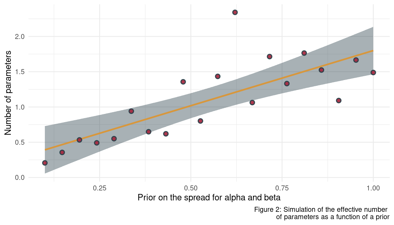
We can see that the number of effective parameters decreases when the prior gets more concentrated. This makes sense as model becomes less flexible in fitting the sample when a prior becomes more concentrated around particular parameter values. With a less flexible model, the effective number of parameters declines.
3.5 Question 7M5
Provide an informal explanation of why informative priors reduce overfitting.
Overfitting means that a model captures too much noise in the data. This noise is not present in new (unseen) data, so the model will fail there. Setting an informative prior is like telling the model to ignore too unrealistic values or at least too lower their leverage. This then leads to an improved predictive performance as the model captures less noise.
3.6 Question 7M6
Provide an informal explanation of why overly informative priors result in underfitting.
If the priors are too concentrated, we tell the model to ignore real patterns in the data. This then reduces predictive performance.
4 Hard practices
4.1 Question 7H1
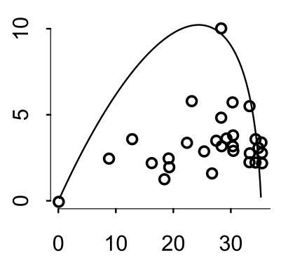
In 2007,The Wall Street Journal published an editorial (“We’re Number One, Alas”) with a graph of corporate tax rates in 29 countries plotted against tax revenue. A badly fit curve was drawn in (reconstructed at right), seemingly by hand, to make the argument that the relationship between tax rate and tax revenue increases and then declines, such that higher tax rates can actually produce less tax revenue. I want you to actually fit a curve to these data, found in data(Laffer). Consider models that use tax rate to predict tax revenue. Compare, using WAIC or PSIS, a straight-line model to any curved models you like. What do you conclude about the relationship between tax rate and tax revenue?
Let’s load the data and standardize all parameters.
data("Laffer")

dat_laffer <- Laffer %>%
  as_tibble() %>%
  mutate(across(everything(), standardize))
We start with a simple linear regression.
m1 <- alist(
  tax_revenue ~ dnorm(mu, sigma),
  mu <- a + Br*tax_rate,
  a ~ dnorm(0, 0.2),
  Br ~ dnorm(0, 0.5),
  sigma ~ dexp(1)
) %>%
  quap(data = dat_laffer)
Now we increase complexity by using a quadratic function.
m2 <- alist(
  tax_revenue ~ dnorm(mu, sigma),
  mu <- a + Br*tax_rate + Br2*tax_rate^2,
  a ~ dnorm(0, 0.2),
  c(Br, Br2) ~ dnorm(0, 0.5),
  sigma ~ dexp(1)
) %>%
  quap(data = dat_laffer)
And finally the cubic model.
m3 <- alist(
  tax_revenue ~ dnorm(mu, sigma),
  mu <- a + Br*tax_rate + Br2*tax_rate^2 + Br3*tax_rate^3,
  a ~ dnorm(0, 0.2),
  c(Br, Br2, Br3) ~ dnorm(0, 0.5),
  sigma ~ dexp(1)
) %>%
  quap(data = dat_laffer)
We can quickly visualise the WAIC values using the plot(compare()) pipeline.
plot(compare(m1, m2, m3))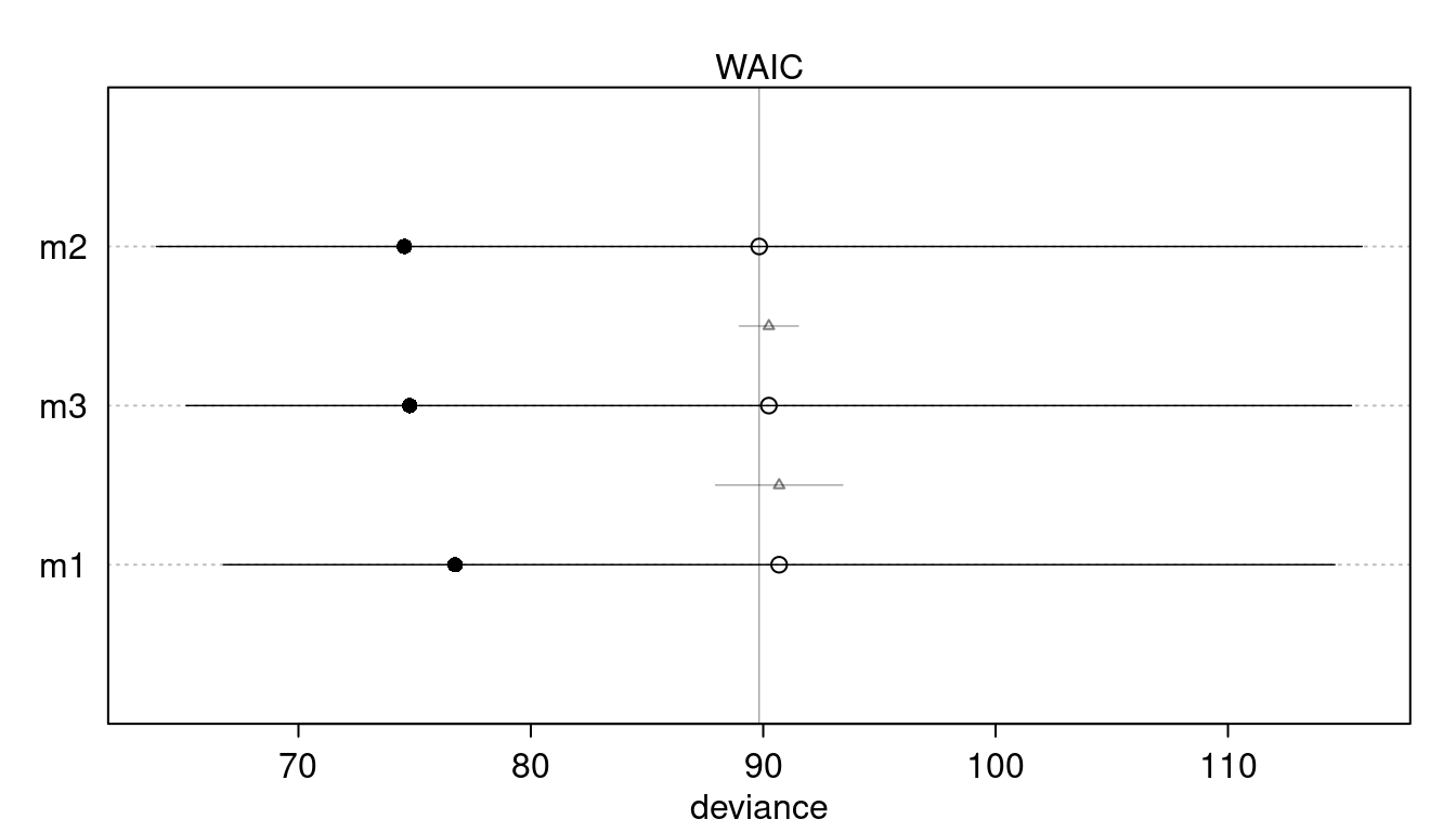
We can already see that there is no support for a particular model. But le’s visualize this a bit more:
N <- 1e3

laffer_fit <- function(model.input, model.type){
    link(model.input, n = N) %>%
    as_tibble() %>%
    pivot_longer(cols = everything(), values_to = "pred_revenue") %>%
    add_column(tax_rate = rep(dat_laffer$tax_rate, N)) %>%
    group_by(tax_rate) %>%
    nest() %>%
    mutate(pred_revenue = map(data, "pred_revenue"),
           mean_revenue = map_dbl(pred_revenue, mean),
           pi = map(pred_revenue, PI),
           lower_pi = map_dbl(pi, pluck(1)),
           upper_pi = map_dbl(pi, pluck(2))) %>%
    add_column(model = model.type) %>%
    select(model, tax_rate, mean_revenue, lower_pi, upper_pi)
}

laffer_fit(m1, "linear") %>%
  full_join(laffer_fit(m2, "quadratic")) %>%
  full_join(laffer_fit(m3, "cubic")) %>%
  ggplot(aes(tax_rate, mean_revenue)) +
  geom_point(aes(tax_rate, tax_revenue),
             colour = grey, alpha = 0.9,
                 data = dat_laffer) +
  geom_ribbon(aes(ymin = lower_pi, ymax = upper_pi,
                  fill = model),
              alpha = 0.3) +
  geom_line(aes(colour = model),
            size = 1.5) +
  scale_colour_manual(values = c(red, yellow, brown)) +
  scale_fill_manual(values = c(red, yellow, brown)) +
  labs(x = "Tax revenue (std)",
       y = "Tax rate (std)",
       caption = "Figure 3: Model predictions for each model.") +
  facet_wrap(~ model) +
  theme_minimal() +
  theme(legend.position = "none")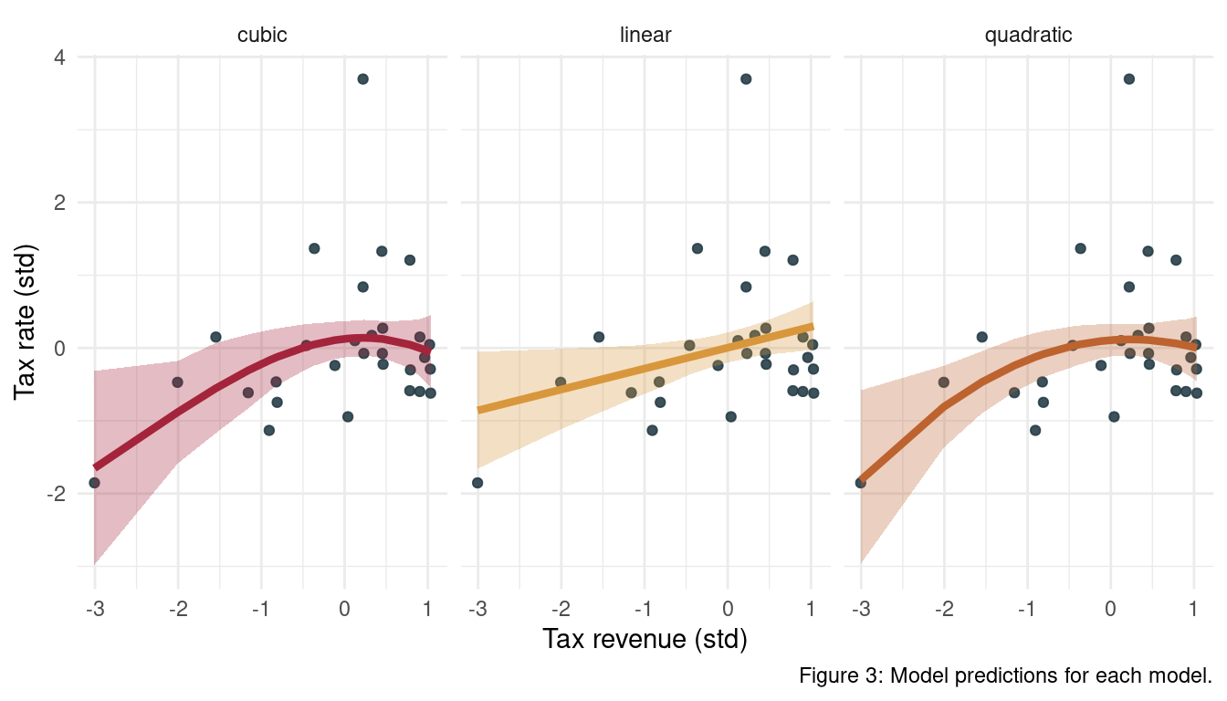
We can see that the uncertainty for each model at the highest revenue is always quite high. Note also that we force a dip at these values for the quadratic model.
4.2 Question 7H2
In the Laffer data, there is one country with a high tax revenue that is an outlier. Use PSIS and WAIC to measure the importance of this outlier in the models you fit in the previous problem. Then use robust regression with a Student’s t distribution to revisit the curve fitting problem. How much does a curved relationship depend upon the outlier point?
Let’s define a function that will help us to get the outlier. The outlier takes a model and returns a data frame with the Pareto-K values, the WAIC penalty, and the model name for each observation in the Laffer data.
get_outlier <- function(model.input, model.type){
  psis_k <- PSIS(model.input, pointwise = TRUE)$k
  waic_pen <- WAIC(model.input, pointwise = TRUE)$penalty
  tibble(psis_k = psis_k, waic_pen = waic_pen, model = model.type)
}
dat_outlier <- get_outlier(m1, model.type = "linear") %>%
full_join(get_outlier(m2, model.type = "quadratic")) %>%
full_join(get_outlier(m3, model.type = "cubic")) Now let’s identify the maximum outlier for each model.
dat_outlier %>%
  group_by(model) %>%
  summarise(max_outlier = which.max(psis_k)) %>%
knitr::kable()| model | max_outlier |
|---|---|
| cubic | 12 |
| linear | 12 |
| quadratic | 12 |
We can see that all models have the 12th observation as an outlier.
dat_laffer[12,]## # A tibble: 1 x 2
## tax_rate tax_revenue
## <dbl> <dbl>
## 1 0.221 3.70We can reproduce the outlier plot from the chapter.
ggplot(aes(psis_k, waic_pen, fill = model),
       data = dat_outlier) +
  geom_point(shape = 21, colour = grey,
             size = 2.5, stroke = 1, alpha = 0.9) +
  scale_fill_manual(values = c(red, yellow, brown)) +
  facet_wrap(~ model) +
  labs(x = "PSIS Pareto K", y = "WAIC penalty",
       caption = "Figure 4: Highly influential points and out-of-sample prediction") +
  theme_bw() +
  theme(legend.position = "none")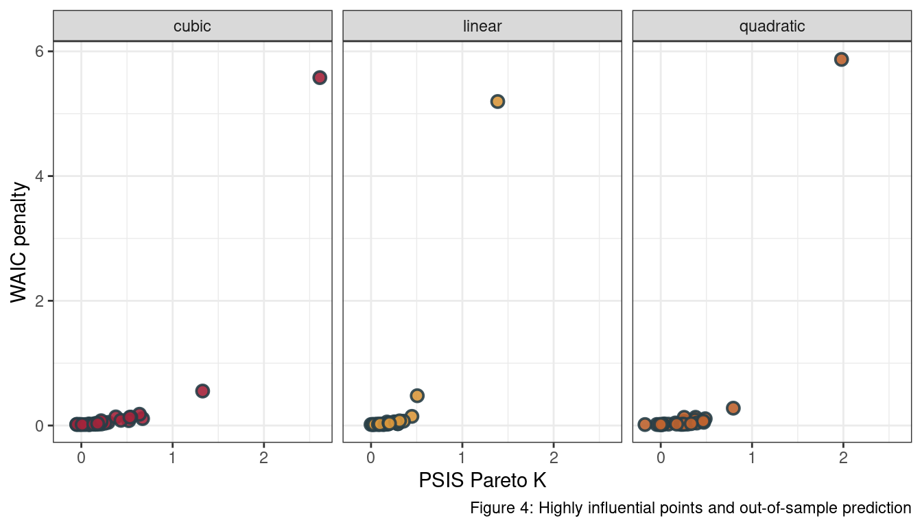
To fit a robust model, we simply use the Student’s T distribution as a likelihood.
m4 <- alist(
  tax_revenue ~ dstudent(2, mu, sigma),
  mu <- a + Br*tax_rate,
  a ~ dnorm(0, 0.2),
  Br ~ dnorm(0, 0.5),
  sigma ~ dexp(1)
) %>%
  quap(data = dat_laffer)
And compare it to the first models.
plot(compare(m1, m2, m3, m4))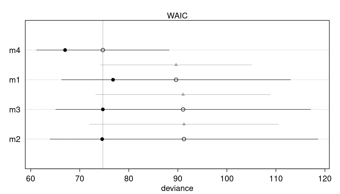
We can see that m4 clearly performs best. Overall, there is no support for a curved relationship.
4.3 Question 7H3
Consider three fictional Polynesian islands. On each there is a Royal Ornithologist charged by the king with surveying the bird population. They have each found the following proportions of 5 important bird species:
dat_island <- tibble("Island" = c("Island 1", "Island 2", "Island 3"),
       "Species A" = c(0.2, 0.8, 0.05),
       "Species B" = c(0.2, 0.1, 0.15),
       "Species C" = c(0.2, 0.05, 0.7),
       "Species D" = c(0.2, 0.025, 0.05),
       "Species E" = c(0.2, 0.025, 0.05))

dat_island %>%
knitr::kable()| Island | Species A | Species B | Species C | Species D | Species E |
|---|---|---|---|---|---|
| Island 1 | 0.20 | 0.20 | 0.20 | 0.200 | 0.200 |
| Island 2 | 0.80 | 0.10 | 0.05 | 0.025 | 0.025 |
| Island 3 | 0.05 | 0.15 | 0.70 | 0.050 | 0.050 |
Notice that each row sums to 1, all the birds. This problem has two parts. It is not computationally complicated. But it is conceptually tricky. First, compute the entropy of each island’s bird distribution.Interpret these entropy values. Second, use each island’s bird distribution to predict the other two.This means to compute the K-L Divergence of each island from the others, treating each island as if it were a statistical model of the other islands. You should end up with 6 different K-L Divergence values. Which island predicts the others best? Why?
To calculate the entropy for each island, we first need to bring the data into a longer format.
dat_island_long <- dat_island %>%
  janitor::clean_names() %>%
  pivot_longer(cols = -island, names_to = "species", values_to = "proportion")
Now we can use the inf_entropy function from practice 7E2 to get the entropy for each island.
dat_island_long %>%
  group_by(island) %>%
  summarise(entropy = inf_entropy(proportion)) %>%
  mutate(across(is.numeric, round, 2)) %>%
knitr::kable()| island | entropy |
|---|---|
| Island 1 | 1.61 |
| Island 2 | 0.74 |
| Island 3 | 0.98 |
Now how to interpret this values. Imagine we throw all birds of an island in a bag, ending with 3 bags full of birds. Entropy is just a measure for how uncertain we are which species we would get, if we grab a random bird from the bag. In the first bag, Island 1, all species are distributed equally and we just have no idea which species we would grab. The entropy is high. On the other hand, the second bag from island 2 is full of ‘species a’ so we are quite certain that we would grab this species. The entropy is hence quite low.
For the second part, we need to apply the Kullback-Leibler divergence, which is given as \[D_{KL}(p,q) = \sum_i(p_i log(p_i) - log(q_i))\]
Or, in R code:
kl_divergence <- function(p,q) sum(p*(log(p)-log(q)))We just need a bit of data wrangling and can then apply kl_divergence for each comparison.
dat_island_long %>%
  select(-species) %>%
  group_by(island) %>%
  nest() %>%
  pivot_wider(names_from = island, values_from = data) %>%
  janitor::clean_names() %>%
  mutate(one_vs_two = map2_dbl(island_1, island_2, kl_divergence),
         two_vs_one = map2_dbl(island_2, island_1, kl_divergence),
         one_vs_three = map2_dbl(island_1, island_3, kl_divergence),
         three_vs_one = map2_dbl(island_3, island_1, kl_divergence),
         two_vs_three = map2_dbl(island_2, island_3, kl_divergence),
         three_vs_two = map2_dbl(island_3, island_2, kl_divergence)
         ) %>%
  select(one_vs_two:three_vs_two) %>%
  pivot_longer(cols = everything(), names_to = "Comparison", values_to = "KL Divergence") %>%
knitr::kable()| Comparison | KL Divergence |
|---|---|
| one_vs_two | 0.9704061 |
| two_vs_one | 0.8664340 |
| one_vs_three | 0.6387604 |
| three_vs_one | 0.6258376 |
| two_vs_three | 2.0109142 |
| three_vs_two | 1.8388452 |
Read the first row as “going from island 1 to island 2 has a divergence of 0.97”. We can see that starting at island 1 results in the overall lowest divergence values, due to the high entropy. If you are used to draw your birds from a bag 1 (from island 1), you are not very surprised of the results from drawing from the other bags. And now I think the bag metaphor reaches its limits.

Anyways, Island 1 predicts the other islands best.
4.4 Question 7H4
Recall the marriage, age, and happiness collider bias example from Chapter 6. Run models m6.9 and m6.10 again. Compare these two models using WAIC (or LOO, they will produce identical results). Which model is expected to make better predictions? Which model provides the correct causal inference about the influence of age on happiness? Can you explain why the answers to these two questions disagree?
First, we need to rerun the simulation to get the data and clean it. More detail is given in chapter 6.
dat_happy <- sim_happiness(seed=1977, N_years=1000)

dat_happy <- dat_happy %>%
  as_tibble() %>%
  filter(age > 17) %>%
  mutate(age = (age - 18)/ (65 -18)) %>%
  mutate(mid = married +1)
Now we can rerun each model.
m6.9 <- alist(
  happiness ~ dnorm( mu , sigma ),
  mu <- a[mid] + bA*age,
  a[mid] ~ dnorm( 0 , 1 ),
  bA ~ dnorm( 0 , 2 ),
  sigma ~ dexp(1)) %>%
  quap(data = dat_happy)

m6.10 <- alist(
  happiness ~ dnorm( mu , sigma ),
  mu <- a + bA*age,
  a ~ dnorm( 0 , 1 ),
  bA ~ dnorm( 0 , 2 ),
  sigma ~ dexp(1)) %>%
  quap(data = dat_happy)
And then we just apply WAIC for both models.
c(m6.9, m6.10) %>%
  map_dfr(WAIC) %>%
  add_column(model = c("m6.9", "m6.10"), .before = 1) %>%
knitr::kable()| model | WAIC | lppd | penalty | std_err |
|---|---|---|---|---|
| m6.9 | 2713.971 | -1353.247 | 3.738532 | 37.54465 |
| m6.10 | 3101.906 | -1548.612 | 2.340445 | 27.74379 |
WAIC favours the model with the collider bias. This is because WAIC cares about predictive power, not causal association. It just doesn’t care that age is not causing happiness. However, the (non-causal but still present)
association between age and happiness results in improved predictions. That’s why WAIC selects the model containing the collider path. This just shows that we shouldn’t use model comparison without a causal model.
4.5 Question 7H5
Revisit the urban fox data, data(foxes), from the previous chapter’s practice problems. Use WAIC or PSIS based model comparison on five different models, each using weight as the outcome, and containing these sets of predictor variables:
- avgfood + groupsize + area
- avgfood + groupsize
- groupsize + area
- avgfood
- area
Can you explain the relative differences in WAIC scores, using the fox DAG from last week’s home-work? Be sure to pay attention to the standard error of the score differences (dSE).
First, reload the data and standardise both the predictors and the outcome.
data("foxes")

dat_foxes <- foxes %>%
  as_tibble() %>%
  mutate(across(-group, standardize))
Now we can fit a model for each description above:
m1 <- alist(
  weight ~ dnorm(mu, sigma),
  mu <- a + Bf*avgfood + Bg*groupsize + Ba*area,
  a ~ dnorm(0, 0.2),
  c(Bf, Bg, Ba) ~ dnorm(0, 0.5),
  sigma ~ dexp(1)) %>%
  quap(data = dat_foxes)

m2 <- alist(
  weight ~ dnorm(mu, sigma),
  mu <- a + Bf*avgfood + Bg*groupsize,
  a ~ dnorm(0, 0.2),
  c(Bf, Bg) ~ dnorm(0, 0.5),
  sigma ~ dexp(1)) %>%
  quap(data = dat_foxes)

m3 <- alist(
  weight ~ dnorm(mu, sigma),
  mu <- a + Bg*groupsize + Ba*area,
  a ~ dnorm(0, 0.2),
  c(Bg, Ba) ~ dnorm(0, 0.5),
  sigma ~ dexp(1)) %>%
  quap(data = dat_foxes)

m4 <- alist(
  weight ~ dnorm(mu, sigma),
  mu <- Bf*avgfood,
  a ~ dnorm(0, 0.2),
  Bf ~ dnorm(0, 0.5),
  sigma ~ dexp(1)) %>%
  quap(data = dat_foxes)

m5 <- alist(
  weight ~ dnorm(mu, sigma),
  mu <- a + Ba*area,
  a ~ dnorm(0, 0.2),
  Ba ~ dnorm(0, 0.5),
  sigma ~ dexp(1)) %>%
  quap(data = dat_foxes)
And then compare them using WAIC.
compare(m1, m2, m3, m4, m5) %>%
  as_tibble(rownames = "model") %>%
  mutate(across(is.numeric, round, 2)) %>%
knitr::kable()| model | WAIC | SE | dWAIC | dSE | pWAIC | weight |
|---|---|---|---|---|---|---|
| m1 | 322.88 | 16.28 | 0.00 | NA | 4.66 | 0.46 |
| m3 | 323.90 | 15.68 | 1.01 | 2.90 | 3.72 | 0.28 |
| m2 | 324.13 | 16.14 | 1.24 | 3.60 | 3.86 | 0.25 |
| m4 | 331.58 | 13.67 | 8.70 | 7.21 | 1.50 | 0.01 |
| m5 | 333.72 | 13.79 | 10.84 | 7.24 | 2.65 | 0.00 |
Remember the DAG from last chapter:
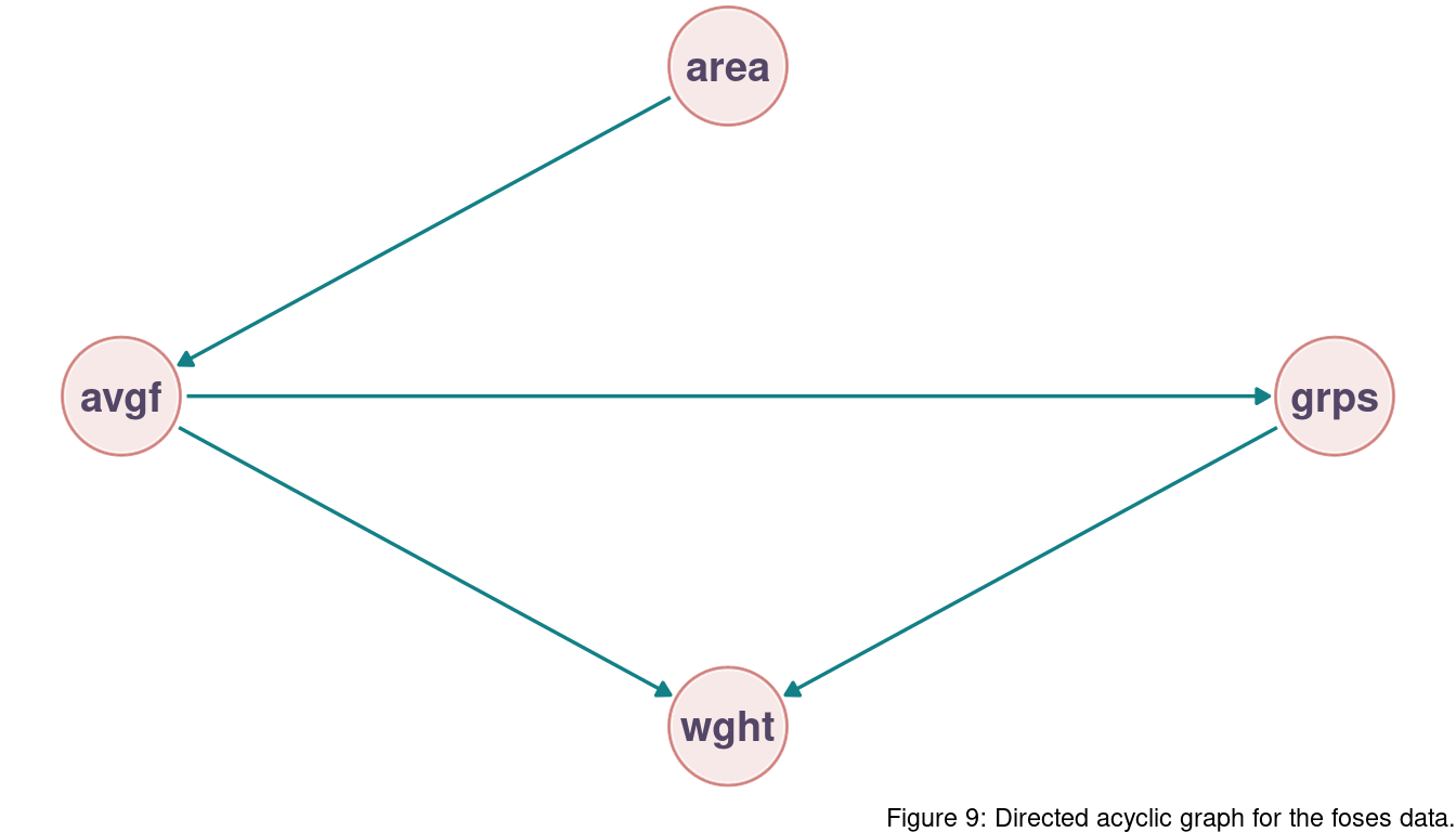
There is no support for the preference of a particular model. But we can see that m1, m2, and m3 are grouped together based on AIC as well as m4 and m5. Following the DAG, as long as we include the groupsize path, it does not make a difference if we use area or avgfood. They encapsulate the same information, and WAIC hence returns a similar value. m4 and m5 both don’t include groupsize. But as avgfood and area contain mostly the same information, they both show similar WAIC estimates.
5 Summary
While reading through this chapter, I had some major problems to understand the complex concepts. But now, I am really happy to experience some mechanistic understanding of model comparison approaches. And even better, I can now casually talk about information entropy, adding new fancy words to my vocabulary.
sessionInfo()## R version 4.0.3 (2020-10-10)
## Platform: x86_64-pc-linux-gnu (64-bit)
## Running under: Linux Mint 20.1
##
## Matrix products: default
## BLAS: /usr/lib/x86_64-linux-gnu/blas/libblas.so.3.9.0
## LAPACK: /usr/lib/x86_64-linux-gnu/lapack/liblapack.so.3.9.0
##
## locale:
## [1] LC_CTYPE=de_DE.UTF-8 LC_NUMERIC=C
## [3] LC_TIME=de_DE.UTF-8 LC_COLLATE=de_DE.UTF-8
## [5] LC_MONETARY=de_DE.UTF-8 LC_MESSAGES=de_DE.UTF-8
## [7] LC_PAPER=de_DE.UTF-8 LC_NAME=C
## [9] LC_ADDRESS=C LC_TELEPHONE=C
## [11] LC_MEASUREMENT=de_DE.UTF-8 LC_IDENTIFICATION=C
##
## attached base packages:
## [1] parallel stats graphics grDevices utils datasets methods
## [8] base
##
## other attached packages:
## [1] rethinking_2.13 rstan_2.21.2 StanHeaders_2.21.0-7
## [4] forcats_0.5.0 stringr_1.4.0 dplyr_1.0.3
## [7] purrr_0.3.4 readr_1.4.0 tidyr_1.1.2
## [10] tibble_3.0.5 ggplot2_3.3.3 tidyverse_1.3.0
##
## loaded via a namespace (and not attached):
## [1] nlme_3.1-151 matrixStats_0.57.0 fs_1.5.0 lubridate_1.7.9.2
## [5] httr_1.4.2 tools_4.0.3 backports_1.2.1 utf8_1.1.4
## [9] R6_2.5.0 DBI_1.1.1 mgcv_1.8-33 colorspace_2.0-0
## [13] withr_2.4.1 tidyselect_1.1.0 gridExtra_2.3 prettyunits_1.1.1
## [17] processx_3.4.5 curl_4.3 compiler_4.0.3 cli_2.2.0
## [21] rvest_0.3.6 xml2_1.3.2 labeling_0.4.2 bookdown_0.21
## [25] scales_1.1.1 mvtnorm_1.1-1 callr_3.5.1 digest_0.6.27
## [29] rmarkdown_2.6 pkgconfig_2.0.3 htmltools_0.5.1.1 dbplyr_2.0.0
## [33] highr_0.8 rlang_0.4.10 readxl_1.3.1 rstudioapi_0.13
## [37] shape_1.4.5 generics_0.1.0 farver_2.0.3 jsonlite_1.7.2
## [41] inline_0.3.17 magrittr_2.0.1 loo_2.4.1 Matrix_1.3-2
## [45] Rcpp_1.0.6 munsell_0.5.0 fansi_0.4.2 lifecycle_0.2.0
## [49] stringi_1.5.3 yaml_2.2.1 snakecase_0.11.0 MASS_7.3-53
## [53] pkgbuild_1.2.0 grid_4.0.3 crayon_1.3.4 lattice_0.20-41
## [57] haven_2.3.1 splines_4.0.3 hms_1.0.0 knitr_1.30
## [61] ps_1.5.0 pillar_1.4.7 codetools_0.2-18 stats4_4.0.3
## [65] reprex_1.0.0 glue_1.4.2 evaluate_0.14 blogdown_1.1
## [69] V8_3.4.0 RcppParallel_5.0.2 modelr_0.1.8 vctrs_0.3.6
## [73] cellranger_1.1.0 gtable_0.3.0 assertthat_0.2.1 xfun_0.20
## [77] janitor_2.1.0 broom_0.7.3 coda_0.19-4 ellipsis_0.3.1