Introduction
I have a very weird relationship to statistics. Even though I was very bad at maths, I decided to study geosciences. I somehow managed to get through the Bachelor maths exams. For some reason, I then proceeded with a shiny new Master program called Analytical Paleobiology that was build around the R programming software and a lot of statistics (it’s an amazing research-oriented program with lots of fossils, stats and outreach courses). During the first lectures, we learned about frequentist null hypothesis significance testing and p-values. It was very confusing, and it is still today. We also learned how to use statistical tests such as a t-test or an ANOVA. It was even more confusing. We’ve got told that these tests are small little black-boxes and that we should not trust them. Then every one just proceeded to work with those black boxes, completely trusting them.
During that Master program I found my passion for stats and programming. Since then, I have read a lot of statistic textbooks and blogs, something that I could never explain my former self that disliked maths. With all this amazing new knowledge, a few things cleared up for me:
- frequentist null hypothesis testing makes no sense
- p-values make no sense
- statistical tests are just regression in disguise
I somehow managed to avoid (1) and (2) by using resampling and permutation methods, and by sticking to effect sizes instead of p-values. Lately, I started to work with Bayesian estimates, completely ditching the frequentist approach (and I will never look back). But statistical tests are still important in my daily work-flow and I simply don’t want to use black boxes anymore. So, basically as a resource to future me, I decided to start a series of blog posts on statistical tests. In each post, I will cover one commonly used statistical test and show that it’s just a regression (and that you get much more power if you express the test as a regression model). I will then proceed to fit a Bayesian regression model for each test, because as John Kruschke states it in the amazing paper Bayesian Estimation Supersedes the t Test(Kruschke 2013):
Some people may wonder which approach, Bayesian or NHST, is more often correct. This question has limited applicability because in real research we never know the ground truth; all we have is a sample of data. If we knew the ground truth, against which to compare the conclusion from the statistical analysis, we would not bother to collect the data. If the question of correctness is instead asked of some hypothetical data generator, the assessment is confined to that particular distribution of simulated data, which likely has only limited resemblance to real-world data encountered across research paradigms. Therefore, instead of asking which method is more often correct in some hypothetical world of simulated data, the relevant question is asking which method provides the richest, most informative, and meaningful results for any set of data. The answer is always Bayesian estimation.
Additionally, using Bayesian estimation, we can quickly escape the omnipresent assumption of normality of many statistical tests. I will start in this blog post with the one sample t-test.
One sample t-test
When to use
If you have one sample of measurements and you want to estimate the central tendency of this sample (e.g. the mean) compared to a specific value. Assume I want to test whether all males from my family tend to be smaller than the average human male. If heights across my male family members are normally distributed, I can use the one sample t-test.
Assumptions
Your sample should have the following characteristics:
- continuous (not discrete)
- normally distributed
- a random sample from its population with each individual in the population having an equal probability of being selected in the sample
As a regression
All we need is a regression that approximates the mean of the sample. Back in high-school, we learned that the intercept of a regression line goes through the mean of the data. So all we need is a regression with an intercept and nothing else We can state this as \[\mu = \alpha\] where \(\alpha\) is the intercept and \(\mu\) the height of each individual. Note that the t-test assumes that height is normally distributed, which we can express as \[height \sim Normal(\mu, \sigma)\]
Comparing the test to the regression
The data
First, we will simulate some data for my male family members height. By simulating the data, we know the true values and can therefore see how each method performs.
set.seed(1708)
dat_height <- rnorm(100, 160, 2)

head(dat_height)
## [1] 162.0337 159.4832 157.5617 158.4347 159.5004 161.0900We just generated 100 height values from a normal distribution with mean 160 cm and a standard deviation of 2. Now we just need a value for the average height of all males. Google says that “The global mean height of adult men born in 1996 is 171 centimeters (cm)”.
The black box
Here’s how you fit the one sample t-test in R:
result_ttest <- t.test(dat_height, mu = 171)We just feed in our data and define the value to which the sample mean should be compared to using mu = 171. The output of this function is very verbose and it’s really painful to extract any values from it.
result_ttest##
## One Sample t-test
##
## data: dat_height
## t = -54.239, df = 99, p-value < 2.2e-16
## alternative hypothesis: true mean is not equal to 171
## 95 percent confidence interval:
## 159.4753 160.2887
## sample estimates:
## mean of x
## 159.882We get a p-value as output that states the probability to get a value of 159.8819784 cm (the mean from my male family members) if the true mean would be 171 cm (average male). The p-value is very low, certainly below many commonly used thresholds, so we could reject the null hypothesis. Are you already confused? Let’s focus on the effect size instead. The mean of my male family members is 159.8819784, and those members are therefore 11.1180216 cm (171 - 159.882 cm) smaller as the average male. As we get a confidence interval for the mean as well, we can transform it to a difference estimate:
ci_ttest <- result_ttest$conf.int %>%
  as.vector()
171 - ci_ttest
## [1] 11.52475 10.71130So male members from my family are 11.12 cm smaller than the average human male, with a 95% CI of [11.52, 10.71].
The regression
To fit a linear regression in R with just an intercept, we can use the formula sample ~ 1. But with this formula, any output that we get compares the mean to a threshold of 0. But we want it to be compared to a threshold of 171, the average human males height. So we need to subtract 170 from each sample first.
result_lm <- lm(dat_height - 171 ~ 1) A real cool thing with this regression approach is that we get the direct difference in means. Let’s take a look:
summary(result_lm)##
## Call:
## lm(formula = dat_height - 171 ~ 1)
##
## Residuals:
## Min 1Q Median 3Q Max
## -4.694 -1.292 0.074 1.094 6.198
##
## Coefficients:
## Estimate Std. Error t value Pr(>|t|)
## (Intercept) -11.118 0.205 -54.24 <2e-16 ***
## ---
## Signif. codes: 0 '***' 0.001 '**' 0.01 '*' 0.05 '.' 0.1 ' ' 1
##
## Residual standard error: 2.05 on 99 degrees of freedomThe p-value is similarly small and the difference is equal to the one sample t-test approach: My male family members are on average 11.12 cm smaller. We can get the confidence intervals with confint().
confint(result_lm)## 2.5 % 97.5 %
## (Intercept) -11.52475 -10.7113Coolio, we obviously get the same results. It seems like the one sample t-test is just a regression in disguise.
Bayesian regression
Now we get to the gold standard, the Bayesian estimation. I will use the brms package for that, which is R’s interface to the Stan language, using a Hamiltonian Markov Chain Monte Carlo and the Nuts sampler. Or as Andrew Heiss stated it in one of his blog posts:
… all the cool kids are using Stan.
library(brms)
options(mc.cores = parallel::detectCores())  # Use all cores
For Bayesian analysis, we can additionally set a prior on the intercept. I will not go into detail, but notice that we can help the model to run by using our knowledge. We do this by setting a weakly informative prior on the intercept with a normal distribution with a mean of 170 and a standard deviation of 3. Why these specific values? Because most males I have seen in my life fall within this range, and it is just reasonable to assume that our sample has similar values. Either way, the prior is so broad that it is easily overwhelmed by the data (it listens to the data), but the model does not assume some very unrealistic values like a height of thousand meters for a human male, or even negative values. We can even visualize the prior:
tibble(height = rnorm(1e5, 170, 10)) %>%
  ggplot(aes(height)) +
  geom_density() +
  theme_minimal()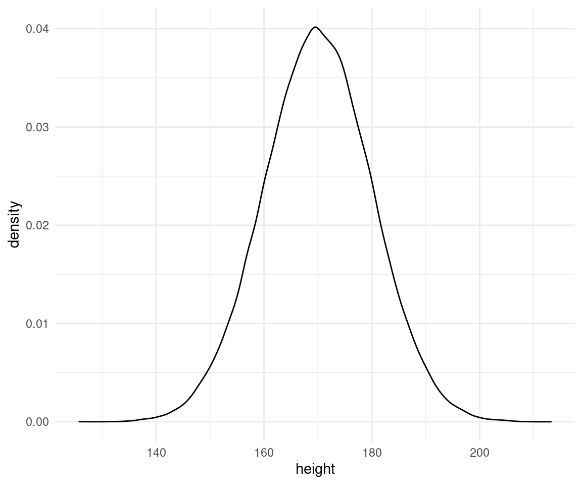
And as we don’t need to fiddle with the meaning of a p-value anymore, I will directly model the mean for our samples using the formula dat_height ~ 1 and then compare these values to the average human male height using posterior samples. Note that I use a standard prior on sigma, which samples from the cauchy distribution.
result_brms <- brm(
  bf(dat_height ~ 1),
  prior = c(set_prior("normal(170, 10)", class = "Intercept"),
            set_prior("cauchy(0, 1)", class = "sigma")),
  chains = 3, iter = 2000, warmup = 1000, data = tibble(dat_height = dat_height))
That’s it. We can get a summary of this model as well:
summary(result_brms)## Family: gaussian
## Links: mu = identity; sigma = identity
## Formula: dat_height ~ 1
## Data: tibble(dat_height = dat_height) (Number of observations: 100)
## Samples: 3 chains, each with iter = 2000; warmup = 1000; thin = 1;
## total post-warmup samples = 3000
##
## Population-Level Effects:
## Estimate Est.Error l-95% CI u-95% CI Rhat Bulk_ESS Tail_ESS
## Intercept 159.89 0.21 159.48 160.29 1.00 2097 1684
##
## Family Specific Parameters:
## Estimate Est.Error l-95% CI u-95% CI Rhat Bulk_ESS Tail_ESS
## sigma 2.06 0.14 1.81 2.37 1.00 2457 1859
##
## Samples were drawn using sampling(NUTS). For each parameter, Bulk_ESS
## and Tail_ESS are effective sample size measures, and Rhat is the potential
## scale reduction factor on split chains (at convergence, Rhat = 1).The Rhat values are equal 1 and the effective sample sizes are large, indicating low autocorrelation. So our model fitted just fine. One great advantage of Bayesian estimation (and Hamiltonian MCMC in particular) is that the model would tell us if something is wrong. The estimate shows the mean for my family members as well as 95% credible intervals. But stop, with frequentist approaches we get only point estimates like these, but with Bayesian estimation we get the whole distribution from the MCMC. Let’s take a look:
result_posterior <- posterior_samples(result_brms)

result_posterior %>%
  ggplot(aes(b_Intercept)) +
  geom_density(colour = "grey20", fill = "firebrick", alpha = 0.8) +
  labs(x = "Mean height", y = NULL) +
theme_minimal() 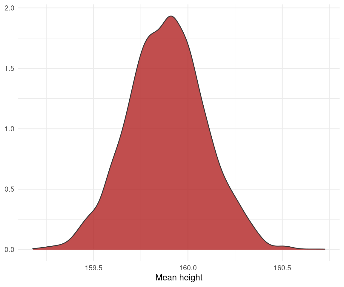
You see that we get aaaall the information we need. What do I mean with that? We get a whole distribution instead of a point estimate (the best guess of ordinary least squares or maximum likelihood) or a range (the confidence interval). So we can take all samples into account and summarize them as we please, using the mean, median, mode and percentile intervals, highest posterior density intervals or credible intervals. We have the power. This is another great advantage of Bayesian estimation. Note also that the model assumes that the response variable (height) comes from a normal distribution. But we are not limited to that (as we are with the t-test and a basic ordinary least squares regression). We can simply change the link function for the response distribution with family = ....
Now to the interpretation: The whole distribution does not include the average human male height of 171 cm, so we can conclude that my male family members are credibly smaller than the average human male. We could even do some Bayesian hypothesis testing to prove this:
hypothesis(result_brms, "Intercept < 171")## Hypothesis Tests for class b:
## Hypothesis Estimate Est.Error CI.Lower CI.Upper Evid.Ratio
## 1 (Intercept)-(171) < 0 -11.11 0.21 -11.44 -10.77 Inf
## Post.Prob Star
## 1 1 *
## ---
## 'CI': 90%-CI for one-sided and 95%-CI for two-sided hypotheses.
## '*': For one-sided hypotheses, the posterior probability exceeds 95%;
## for two-sided hypotheses, the value tested against lies outside the 95%-CI.
## Posterior probabilities of point hypotheses assume equal prior probabilities.As the credible interval does not include zero and the evidence ratio is really high, we can accept the hypothesis that my family male members have a mean height smaller than 171 cm. What did I just say? Accepting a hypothesis is not possible, right? But this is only true for frequentist approaches and not for Bayesian ones. The p-value of a frequentist approach gives us the probability for the data under a null hypothesis \[p(data | N_0)\] Bayesian estimation instead gives us the probability of a hypothesis given the data \[p(N_0 | data)\] This is basically what we wanted from the beginning.
Comparison of all methods
Let’s compare the estimates of all approaches.
tibble(Model = c("T-Test",
                 "OLS Regression",
                 "Bayesian Regression"),
       Estimate = c(result_ttest$estimate - 171,
                    result_lm$coefficients,
                    fixef(result_brms)[1] - 171),
       Est_Error = c(result_ttest$stderr,
                     summary(result_lm)$coefficients[2],
                     fixef(result_brms)[2]),
       Lower_CI = c(result_ttest$conf.int[1] -171,
                    confint(result_lm)[1],
                    fixef(result_brms)[3] - 171),
       Upper_CI = c(result_ttest$conf.int[2] -171,
                    confint(result_lm)[2],
                    fixef(result_brms)[4] - 171),
       p_Value = c(result_ttest$p.value,
                   summary(result_lm)$coefficients[4],
                   NA)) %>%
  mutate(across(Estimate:Upper_CI, round, 2)) %>%
knitr::kable(digits = 100)| Model | Estimate | Est_Error | Lower_CI | Upper_CI | p_Value |
|---|---|---|---|---|---|
| T-Test | -11.12 | 0.20 | -11.52 | -10.71 | 1.928903e-75 |
| OLS Regression | -11.12 | 0.20 | -11.52 | -10.71 | 1.928903e-75 |
| Bayesian Regression | -11.11 | 0.21 | -11.52 | -10.71 | NA |
That looks very good. Note that the CI is a 95% confidence interval for the frequentist approaches, and a 95% credible interval for the Bayesian estimation. To sum this up: The t-test is nothing but a regression, and we can always do better than a OLS regression by using a Bayesian regression. Why? Because in stark contrast to all frequentist approaches, it gives us the answers we want.
sessionInfo()## R version 4.0.4 (2021-02-15)
## Platform: x86_64-pc-linux-gnu (64-bit)
## Running under: Linux Mint 20.1
##
## Matrix products: default
## BLAS: /usr/lib/x86_64-linux-gnu/blas/libblas.so.3.9.0
## LAPACK: /usr/lib/x86_64-linux-gnu/lapack/liblapack.so.3.9.0
##
## locale:
## [1] LC_CTYPE=de_DE.UTF-8 LC_NUMERIC=C
## [3] LC_TIME=de_DE.UTF-8 LC_COLLATE=de_DE.UTF-8
## [5] LC_MONETARY=de_DE.UTF-8 LC_MESSAGES=de_DE.UTF-8
## [7] LC_PAPER=de_DE.UTF-8 LC_NAME=C
## [9] LC_ADDRESS=C LC_TELEPHONE=C
## [11] LC_MEASUREMENT=de_DE.UTF-8 LC_IDENTIFICATION=C
##
## attached base packages:
## [1] stats graphics grDevices utils datasets methods base
##
## other attached packages:
## [1] brms_2.15.0 Rcpp_1.0.6 forcats_0.5.0 stringr_1.4.0
## [5] dplyr_1.0.3 purrr_0.3.4 readr_1.4.0 tidyr_1.1.2
## [9] tibble_3.0.5 ggplot2_3.3.3 tidyverse_1.3.0
##
## loaded via a namespace (and not attached):
## [1] minqa_1.2.4 colorspace_2.0-0 ellipsis_0.3.1
## [4] ggridges_0.5.3 rsconnect_0.8.16 markdown_1.1
## [7] base64enc_0.1-3 fs_1.5.0 rstudioapi_0.13
## [10] farver_2.0.3 rstan_2.21.2 DT_0.17
## [13] fansi_0.4.2 mvtnorm_1.1-1 lubridate_1.7.9.2
## [16] xml2_1.3.2 codetools_0.2-18 bridgesampling_1.0-0
## [19] splines_4.0.4 knitr_1.30 shinythemes_1.2.0
## [22] bayesplot_1.8.0 projpred_2.0.2 jsonlite_1.7.2
## [25] nloptr_1.2.2.2 broom_0.7.3 dbplyr_2.0.0
## [28] shiny_1.6.0 compiler_4.0.4 httr_1.4.2
## [31] backports_1.2.1 assertthat_0.2.1 Matrix_1.3-2
## [34] fastmap_1.1.0 cli_2.2.0 later_1.1.0.1
## [37] prettyunits_1.1.1 htmltools_0.5.1.1 tools_4.0.4
## [40] igraph_1.2.6 coda_0.19-4 gtable_0.3.0
## [43] glue_1.4.2 reshape2_1.4.4 V8_3.4.0
## [46] cellranger_1.1.0 vctrs_0.3.6 nlme_3.1-152
## [49] blogdown_1.1 crosstalk_1.1.1 xfun_0.20
## [52] ps_1.5.0 lme4_1.1-26 rvest_0.3.6
## [55] mime_0.9 miniUI_0.1.1.1 lifecycle_0.2.0
## [58] gtools_3.8.2 statmod_1.4.35 MASS_7.3-53.1
## [61] zoo_1.8-8 scales_1.1.1 colourpicker_1.1.0
## [64] hms_1.0.0 promises_1.1.1 Brobdingnag_1.2-6
## [67] parallel_4.0.4 inline_0.3.17 shinystan_2.5.0
## [70] curl_4.3 gamm4_0.2-6 yaml_2.2.1
## [73] gridExtra_2.3 StanHeaders_2.21.0-7 loo_2.4.1
## [76] stringi_1.5.3 highr_0.8 dygraphs_1.1.1.6
## [79] pkgbuild_1.2.0 boot_1.3-27 rlang_0.4.10
## [82] pkgconfig_2.0.3 matrixStats_0.57.0 evaluate_0.14
## [85] lattice_0.20-41 labeling_0.4.2 rstantools_2.1.1
## [88] htmlwidgets_1.5.3 processx_3.4.5 tidyselect_1.1.0
## [91] plyr_1.8.6 magrittr_2.0.1 bookdown_0.21
## [94] R6_2.5.0 generics_0.1.0 DBI_1.1.1
## [97] pillar_1.4.7 haven_2.3.1 withr_2.4.1
## [100] mgcv_1.8-33 xts_0.12.1 abind_1.4-5
## [103] modelr_0.1.8 crayon_1.3.4 rmarkdown_2.6
## [106] grid_4.0.4 readxl_1.3.1 callr_3.5.1
## [109] threejs_0.3.3 reprex_1.0.0 digest_0.6.27
## [112] xtable_1.8-4 httpuv_1.5.5 RcppParallel_5.0.2
## [115] stats4_4.0.4 munsell_0.5.0 shinyjs_2.0.0