Introduction
This is the second post for my series on statistical tests as regression models. I want to show that each classical stats test such as an ANOVA or a t-test are just linear regression models in disguise. After showing this concept for each test, I aim to build a Bayesian regression for each that supersedes both the classical test and the frequentist regression approach. You can find the other parts from the statistical tests as regression series here.
In this post, I will cover the non-parametric sibling of the one sample t-test, the Wilcoxon signed-rank test. I will use this opportunity to introduce rank-transformations for non-normal data.
Wilcoxon signed-rank test
When to use
Similar to the one sample t-test (which I have covered in another blog post), the Wilcoxon signed-rank test can be applied to estimate the central tendency of a sample (e.g. the mean) compared to a specific value. For example, if I want to estimate whether the average IQ of my colleagues at University Bayreuth is above the overall average IQ of 100. The good thing about the Wilcoxon signed-rank test compared to the t-test is the relaxation of the assumption of normality. If you have evidence that the distribution of the response variable in your sample is non-normally distributed, you typically apply the Wilcoxon signed-rank test.
How does it work?
The one sample t-test belongs to the parametric tests. That means that the test makes assumption about your data, and only under those assumptions the test will return reliable results. The Wilcoxon signed-rank test on the other hand is non-parametric and does not care about the underlying distribution. But how does that work? It turns out that within the black box of the test, all our data get transformed. Before the test is evaluated, the data gets ordered in signed ranks (hence the name). After transformation, the data is more or less Gaussian shaped, and then thrown in a one sample t-test. So the Wilcoxon signed-rank test is just a one sample t-test with some data transformation beforehand. And as we know how the t-test looks as a regression, we can quite easily disentangle the black box of the Wilcoxon test. But first, let’s look at how signed rank transformation works.
Signed rank transformation
If you have some data points, you can order them via their ranks from low to high. In R, you can do this via the rank() function.
dat <- c(1, 5, 3, -2, 20, -5)

dat %>%
  rank()
## [1] 3 5 4 2 6 1The lowest number (-5 in the example) gets assigned the rank 1. Now the signed rank transformation works quite similar. We just take the absolute of the data, rank it and then assign each data point the same sign it has before we took the absolute.
dat %>%
  abs() %>%
  rank() * sign(dat)
## [1] 1.0 4.5 3.0 -2.0 6.0 -4.5But why bother? It turns out that this transformation is able to make a non-normal distribution normally shaped. And this then allows us to apply various parametric tests (you shouldn’t though, but let’s keep that for later). We can show this by sampling from a number of non-normal data, and then try to make them Gaussian shaped by applying the signed-rank transformation.
# simulate data from various distributions
simulated_data <- tibble(log_normal = rlnorm(1e5),
       poisson = rpois(1e5, 10),
       binomial = rbinom(1e5, 10, 0.5),
       exponential = rexp(1e5)) %>%
  pivot_longer(cols = everything(),
               names_to = "distribution",
               values_to = "value")

# plot untransformed data
simulated_data %>%
  ggplot(aes(value)) +
  geom_density(fill = "grey50", colour = "grey10",
               alpha = 0.9) +
  facet_wrap(~distribution, scale = "free") +
  theme_minimal()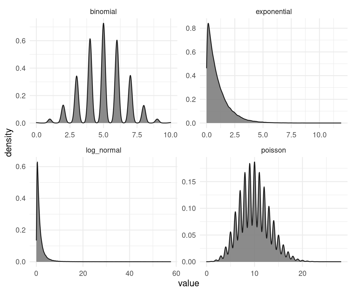
So that’s the un-transformed simulated data. Now let’s try to transform them.
# define the transformation function
signed_rank <-  function(x) {
  sign(x) * rank(abs(x))
}

# apply the transformation to each distribution
simulated_data %>%
  group_by(distribution) %>%
  mutate(trans_value = signed_rank(value)) %>%
  ggplot(aes(trans_value)) +
  geom_density(fill = "grey50", colour = "grey10",
               alpha = 0.9) +
  facet_wrap(~distribution, scale = "free") +
  theme_minimal()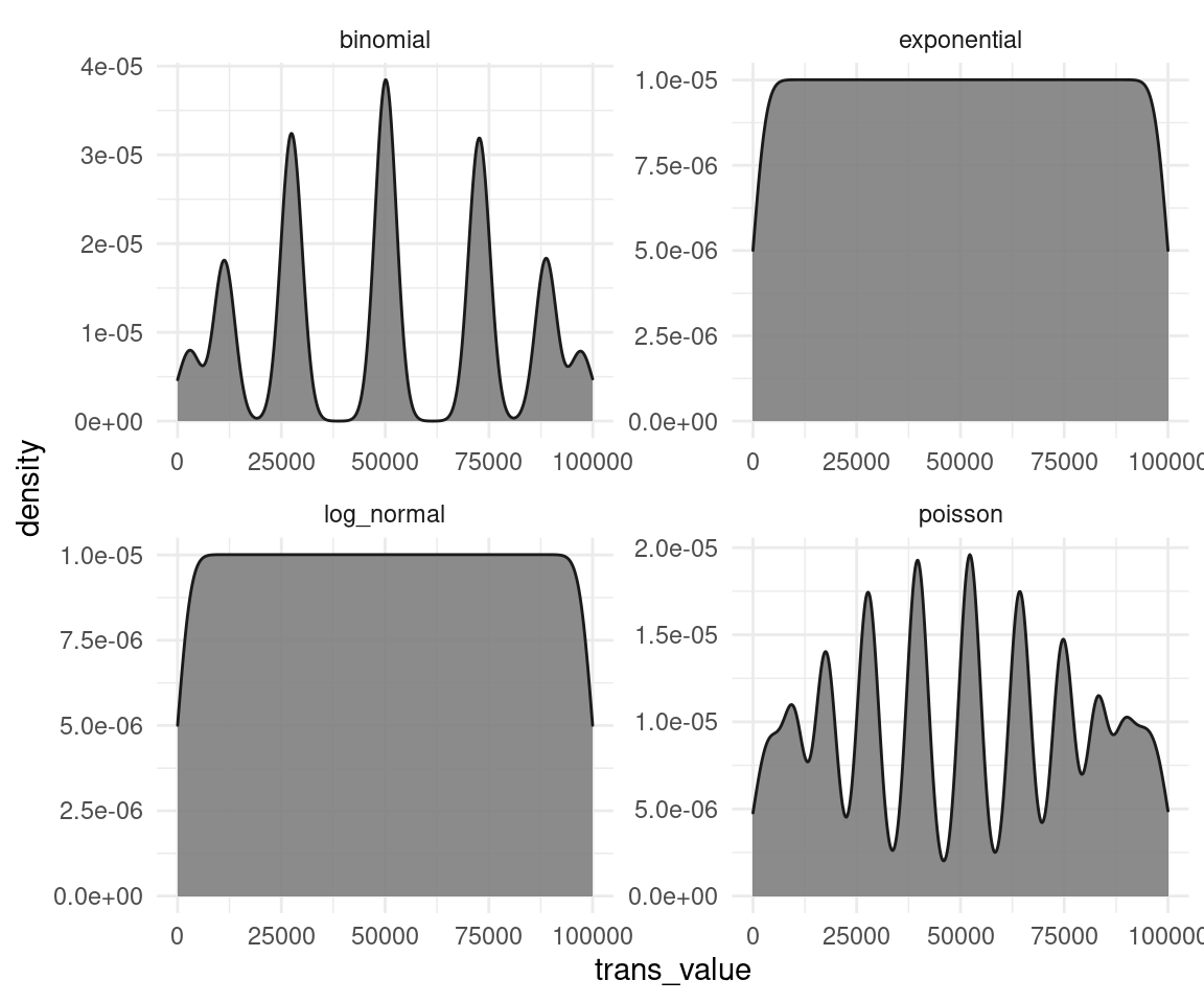
We can see that the transformation does not work properly on all distributions (especially for the binomial and the poisson data). This is because the rank-transformation works only for continuous data, and not for discrete. And on the other distributions, it seems like a mixture of a normal and a uniform distribution. The test is applied as a black box and you don’t see these transformations, and that those transformations might fail. We will see how to overcome these problems with Bayesian estimation later on in this blog. But not only Bayesian estimation is capable to tackle these issues. There are frequentist ways for regression on discrete data as well. But all of this requires thinking, cross-checking, and plotting each step in the analysis. You won’t tackle these issues with a classical test like. Even worse, if you throw the data in such a black box, it won’t even tell you that something is wrong, or that it’s assumptions are violated.
Assumptions
Even though the Wilcoxon signed-rank test relaxes the normality assumption of the one sample t-test, it still relies on a number of assumption.
- continuous (not discrete) and measured on an interval scale
- normally distributed
- a random sample from its population with each individual in the population having an equal probability of being selected in the sample
As a regression
We can simply take the regression formula for the one sample t-test after applying the signed-rank transformation. So all we need is a regression with an intercept and nothing less. We can state this as \[\mu = \alpha\] where \(\alpha\) is the intercept and \(\mu\) the height of each individual.
Comparing the test to the regression
The data
I will generate data for chess games, because according to a stackexchange post, The length of chess games tends to follow a log-normal distribution. If you would plot the data first and realize that it comes from a log-normal, you could easily transform it to a Gaussian curve instead of using rank-transformation. This would then result in an improved estimation compared to the Wilcoxon test. But we will come to that in a second. Here’s the data, with values taken from the stackexchange post:
set.seed(1708)
dat_chess <- rlnorm(1e5, 4.37, 0.45)

dat_chess %>%
  as_tibble() %>%
  ggplot(aes(value)) +
  geom_density(fill = "grey50", colour = "grey10",
               alpha = 0.9) +
  labs(x = "Length of chess game") +
  theme_minimal()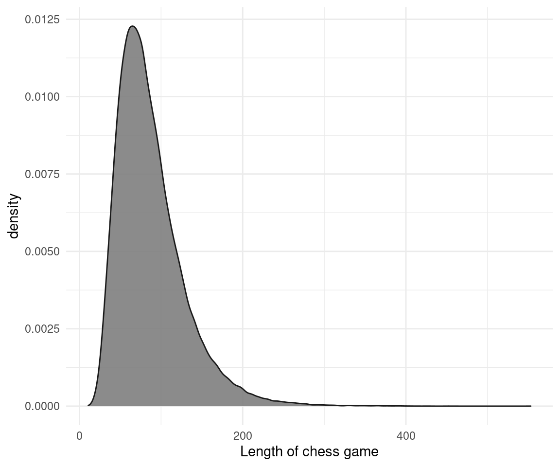
With this much data, all our p-value would be totally small (see the problem?). So I will sample 200 values from this total distribution.
set.seed(1708)
dat_chess <- sample(dat_chess, 200)
Our hypothesis is that the average chess game from this sample takes more than 75 minutes. Why? Because my total play time for online chess averages around this value, and I want to see where I am in terms of chess game longevity.
The black box
We can just throw the data in the Wilcoxon signed-rank test and define the value we want to compare with mu. We can set our hypothesis specified above via alternative = "greater".
wilcox.test(dat_chess, mu = 75, alternative = "greater")##
## Wilcoxon signed rank test with continuity correction
##
## data: dat_chess
## V = 12200, p-value = 0.004361
## alternative hypothesis: true location is greater than 75We get a p-value below a arbitrarily chosen threshold and are hence able to reject the null hypothesis that our sample mean is equal or below 75 minutes. However, we should not stick to p-values and instead report effect sizes and confidence intervals. We can get these for the test by specifying that we want a (non-parametric) confidence interval.
wilcox.test(dat_chess, mu = 75,
            alternative = "greater", conf.int = TRUE)
##
## Wilcoxon signed rank test with continuity correction
##
## data: dat_chess
## V = 12200, p-value = 0.004361
## alternative hypothesis: true location is greater than 75
## 95 percent confidence interval:
## 76.95927 Inf
## sample estimates:
## (pseudo)median
## 80.2828Interestingly, we get an infinite value for the upper bound of the confidence interval. That’s because we conduct a one sided test as we only compare if our sample average is greater. To get a confidence interval on both sides, we need a two sided test.
wilcox_results <- wilcox.test(dat_chess, mu = 75,
                              alternative = "two.sided", conf.int = TRUE)

wilcox_results
##
## Wilcoxon signed rank test with continuity correction
##
## data: dat_chess
## V = 12200, p-value = 0.008722
## alternative hypothesis: true location is not equal to 75
## 95 percent confidence interval:
## 76.30875 84.47312
## sample estimates:
## (pseudo)median
## 80.2828Looks good, the 95% CI does not include my average play time of 75 minutes.
The other black box
Here’s the proof that the Wilcoxon signed-rank test is a one sample t-test with sign-ranked transformed data:
dat_chess %>%
  signed_rank() %>%
  t.test(mu = 75)
##
## One Sample t-test
##
## data: .
## t = 6.2306, df = 199, p-value = 2.717e-09
## alternative hypothesis: true mean is not equal to 75
## 95 percent confidence interval:
## 92.42942 108.57058
## sample estimates:
## mean of x
## 100.5Huh, what happened here? We get different values for the confidence intervals and the estimate. But that’s just because the t-test estimates the mean, while the Wilcoxon test estimates the median. The median is a bit more robust to outliers.
The regression
We realized that the Wilcoxon test estimates the median, and that is a bit harder with frequentist regression. But here’s the regression formula for the mean:
ols_result <- lm(signed_rank(dat_chess) ~ 1)

ols_result
##
## Call:
## lm(formula = signed_rank(dat_chess) ~ 1)
##
## Coefficients:
## (Intercept)
## 100.5confint(ols_result)## 2.5 % 97.5 %
## (Intercept) 92.42942 108.5706This is the same as for the t-test on sign-ranked data. But we are not restricted to model the mean via regression. With the help of a quantile regression, we can model the median instead. But we need the quantreg package for this. Note that the quantreg package uses the sign ranking by default.
library(quantreg)

qr_result <- rq(dat_chess ~ 1)
## Warning in rq.fit.br(x, y, tau = tau, ...): Solution may be nonuniqueqr_result## Call:
## rq(formula = dat_chess ~ 1)
##
## Coefficients:
## (Intercept)
## 77.97497
##
## Degrees of freedom: 200 total; 199 residualWe can get confidence intervals for the median via bootstrapping the standard deviation:
qr_se <- summary(qr_result, se = "boot")[[3]][2] * 1.96

qr_confint <- c(qr_result$coefficients[[1]] - qr_se,
                c(qr_result$coefficients[[1]] + qr_se))
qr_confint
## [1] 73.10056 82.84938Bayesian estimation
The model
We could already see that we get into weird terrain with these parametric and non-parametric stuff. But reverend Bayes comes to the rescue. We can model the whole posterior distribution for our sample and can even verify the null hypothesis, not only reject it. And we are not bound to arbitrary thresholds, but can base our decision on the whole set of information, instead of point estimates. As I am playing chess from time to time, I know that most games are quite short but that some games tend to be extremely long. I have written the stackexchange post mentioned above and therefore have prior knowledge that the duration of chess games is log-normal distributed. We can use this information in the Bayesian model:
library(brms)## Lade nötiges Paket: Rcpp## Loading 'brms' package (version 2.15.0). Useful instructions
## can be found by typing help('brms'). A more detailed introduction
## to the package is available through vignette('brms_overview').##
## Attache Paket: 'brms'## The following object is masked from 'package:stats':
##
## aroptions(mc.cores = parallel::detectCores()) # Use all cores
bayes_result <- brm(
bf(dat_chess ~ 1),
family = "lognormal",
prior = c(set_prior("normal(10, 10)", class = "Intercept")),
chains = 3, iter = 2000, warmup = 1000, data = tibble(dat_chess = dat_chess))## Compiling Stan program...## Start samplingThe model returns the posterior on the log-normal scale, so we should take the exponential for all values of the posterior later on. Note that I have set a rather non-informative prior on the mean. Let’s take a look at the posterior.
result_posterior <- posterior_samples(bayes_result)

result_posterior %>%
  mutate(across(b_Intercept:sigma, exp)) %>%
  ggplot(aes(b_Intercept)) +
  geom_density(colour = "grey20", fill = "coral2", alpha = 0.8) +
  labs(x = "Mean height", y = NULL) +
theme_minimal() 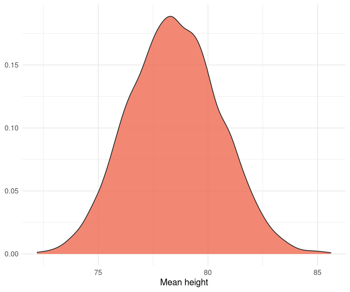
And we can proceed to test our hypothesis:
hyp_test <- result_posterior %>%
  mutate(b_Intercept= exp(b_Intercept)) %>%
  hypothesis("b_Intercept > 75")

hyp_test
## Hypothesis Tests for class :
## Hypothesis Estimate Est.Error CI.Lower CI.Upper Evid.Ratio
## 1 (b_Intercept)-(75) > 0 3.49 2.05 0.21 6.89 23.39
## Post.Prob Star
## 1 0.96 *
## ---
## 'CI': 90%-CI for one-sided and 95%-CI for two-sided hypotheses.
## '*': For one-sided hypotheses, the posterior probability exceeds 95%;
## for two-sided hypotheses, the value tested against lies outside the 95%-CI.
## Posterior probabilities of point hypotheses assume equal prior probabilities.It’s 23.4 times more likely that the average chess game from the sample takes more than 75 minutes, than that the average is less than 75 minutes.
Comparison
As we simulated the data by ourselves, we can compare each method to the true value. We used a value of 4.37 for the log-normal mean, and 0.45 for the log-normal standard deviation. We need to transform the values for each method to the log-normal scale for a proper comparison.
dat_comparison <- tibble(method = c("OLS",
                                    "Quantreg",
                                    "Wilcoxon",
                                    "Bayes"),
       mean = c(ols_result$coefficients[1] %>% log(),
                qr_result$coefficients[1] %>% log(),
                wilcox_results$estimate[1] %>% log(),
                fixef(bayes_result)[1]),
       mean_lower = c(confint(ols_result)[1]%>% log(),
                      qr_confint[1] %>% log(),
                      wilcox_results$conf.int[1]%>% log(),
                      fixef(bayes_result)[3]),
       mean_upper = c(confint(ols_result)[2]%>% log(),
                      qr_confint[2] %>% log(),
                      wilcox_results$conf.int[2]%>% log(),
                      fixef(bayes_result)[4]),
       sd = c(NA,
              summary(qr_result, se = "boot")[[3]][2] %>% log(),
              NA,
              posterior_summary(bayes_result)[2, 1]),
       sd_lower = c(NA,
                    NA,
                    NA,
                    posterior_summary(bayes_result)[2, 3]),
       sd_upper = c(NA,
                    NA,
                    NA,
                    posterior_summary(bayes_result)[2, 4]))


dat_comparison %>%
knitr::kable(digits = 3)| method | mean | mean_lower | mean_upper | sd | sd_lower | sd_upper |
|---|---|---|---|---|---|---|
| OLS | 4.610 | 4.526 | 4.687 | NA | NA | NA |
| Quantreg | 4.356 | 4.292 | 4.417 | 0.896 | NA | NA |
| Wilcoxon | 4.386 | 4.335 | 4.436 | NA | NA | NA |
| Bayes | 4.363 | 4.313 | 4.413 | 0.377 | 0.342 | 0.418 |
We can see that we get a whole posterior on sigma as well with Bayesian estimation. Let’s visualize the comparison with the actual value highlighted in red:
dat_comparison %>%
  ggplot(aes(mean, method,
             xmin = mean_lower,
             xmax = mean_upper)) +
  geom_vline(xintercept = 4.37,
             size = 2, colour = "coral2") +
  geom_pointrange(size = 0.9) +
  labs(x = "Log of the mean duration of chess games",
       y = NULL) +
  theme_minimal()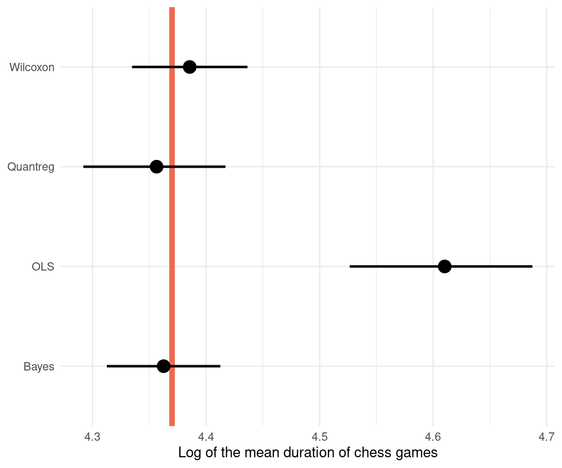
We can transform that to the normal scale by taking the exponential:
dat_comparison %>%
  mutate(across(mean:mean_upper, exp)) %>%
  ggplot(aes(mean, method,
             xmin = mean_lower,
             xmax = mean_upper)) +
  geom_vline(xintercept = exp(4.37),
             size = 2, colour = "coral2") +
  geom_pointrange(size = 0.9) +
  labs(x = "Mean duration of chess games",
       y = NULL) +
  theme_minimal()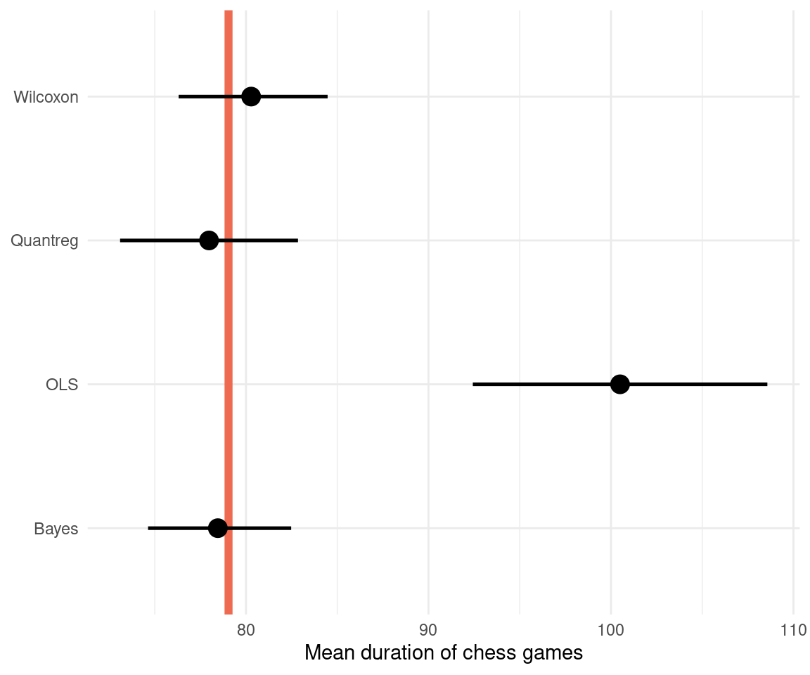
The Bayesian regression performs best, however the Wilcoxon test still is close to the true value, similar to the quantile regression. This shows that when all assumptions are met, the Wilcoxon test can still be a powerful tool. Just don’t use it without knowing what’s going on. We can see that an ordinary least squares regression (OLS) is quite far off, because it models the mean and not the median. It is therefore less robust. And I would assume that the Wilcoxon test in R performs some extra steps and corrections that leads to the better estimate for our data.
Conclusion
The Wilcoxon test performs quite well but is a black box and should not be used. Of cause, if all assumptions are met, it is still fine to use this statistical test. But using Bayesian regression does not only result in better estimation, it gives us all information needed for a valid hypothesis testing and taking decisions with minimizing the expected loss.
sessionInfo()## R version 4.0.4 (2021-02-15)
## Platform: x86_64-pc-linux-gnu (64-bit)
## Running under: Linux Mint 20.1
##
## Matrix products: default
## BLAS: /usr/lib/x86_64-linux-gnu/blas/libblas.so.3.9.0
## LAPACK: /usr/lib/x86_64-linux-gnu/lapack/liblapack.so.3.9.0
##
## locale:
## [1] LC_CTYPE=de_DE.UTF-8 LC_NUMERIC=C
## [3] LC_TIME=de_DE.UTF-8 LC_COLLATE=de_DE.UTF-8
## [5] LC_MONETARY=de_DE.UTF-8 LC_MESSAGES=de_DE.UTF-8
## [7] LC_PAPER=de_DE.UTF-8 LC_NAME=C
## [9] LC_ADDRESS=C LC_TELEPHONE=C
## [11] LC_MEASUREMENT=de_DE.UTF-8 LC_IDENTIFICATION=C
##
## attached base packages:
## [1] stats graphics grDevices utils datasets methods base
##
## other attached packages:
## [1] brms_2.15.0 Rcpp_1.0.6 quantreg_5.83 SparseM_1.78
## [5] forcats_0.5.0 stringr_1.4.0 dplyr_1.0.3 purrr_0.3.4
## [9] readr_1.4.0 tidyr_1.1.2 tibble_3.0.5 ggplot2_3.3.3
## [13] tidyverse_1.3.0
##
## loaded via a namespace (and not attached):
## [1] minqa_1.2.4 colorspace_2.0-0 ellipsis_0.3.1
## [4] ggridges_0.5.3 rsconnect_0.8.16 markdown_1.1
## [7] base64enc_0.1-3 fs_1.5.0 rstudioapi_0.13
## [10] rstan_2.21.2 farver_2.0.3 MatrixModels_0.4-1
## [13] DT_0.17 fansi_0.4.2 mvtnorm_1.1-1
## [16] lubridate_1.7.9.2 xml2_1.3.2 codetools_0.2-18
## [19] bridgesampling_1.0-0 splines_4.0.4 knitr_1.30
## [22] shinythemes_1.2.0 bayesplot_1.8.0 projpred_2.0.2
## [25] jsonlite_1.7.2 nloptr_1.2.2.2 broom_0.7.3
## [28] dbplyr_2.0.0 shiny_1.6.0 compiler_4.0.4
## [31] httr_1.4.2 backports_1.2.1 assertthat_0.2.1
## [34] Matrix_1.3-2 fastmap_1.1.0 cli_2.2.0
## [37] later_1.1.0.1 prettyunits_1.1.1 htmltools_0.5.1.1
## [40] tools_4.0.4 igraph_1.2.6 coda_0.19-4
## [43] gtable_0.3.0 glue_1.4.2 reshape2_1.4.4
## [46] V8_3.4.0 cellranger_1.1.0 vctrs_0.3.6
## [49] nlme_3.1-152 conquer_1.0.2 blogdown_1.1
## [52] crosstalk_1.1.1 xfun_0.20 ps_1.5.0
## [55] lme4_1.1-26 rvest_0.3.6 miniUI_0.1.1.1
## [58] mime_0.9 lifecycle_0.2.0 gtools_3.8.2
## [61] statmod_1.4.35 MASS_7.3-53.1 zoo_1.8-8
## [64] scales_1.1.1 colourpicker_1.1.0 hms_1.0.0
## [67] promises_1.1.1 Brobdingnag_1.2-6 parallel_4.0.4
## [70] inline_0.3.17 shinystan_2.5.0 curl_4.3
## [73] gamm4_0.2-6 yaml_2.2.1 gridExtra_2.3
## [76] StanHeaders_2.21.0-7 loo_2.4.1 stringi_1.5.3
## [79] highr_0.8 dygraphs_1.1.1.6 pkgbuild_1.2.0
## [82] boot_1.3-27 rlang_0.4.10 pkgconfig_2.0.3
## [85] matrixStats_0.57.0 evaluate_0.14 lattice_0.20-41
## [88] rstantools_2.1.1 htmlwidgets_1.5.3 labeling_0.4.2
## [91] processx_3.4.5 tidyselect_1.1.0 plyr_1.8.6
## [94] magrittr_2.0.1 bookdown_0.21 R6_2.5.0
## [97] generics_0.1.0 DBI_1.1.1 pillar_1.4.7
## [100] haven_2.3.1 withr_2.4.1 mgcv_1.8-33
## [103] xts_0.12.1 abind_1.4-5 modelr_0.1.8
## [106] crayon_1.3.4 rmarkdown_2.6 grid_4.0.4
## [109] readxl_1.3.1 callr_3.5.1 threejs_0.3.3
## [112] reprex_1.0.0 digest_0.6.27 xtable_1.8-4
## [115] httpuv_1.5.5 RcppParallel_5.0.2 stats4_4.0.4
## [118] munsell_0.5.0 shinyjs_2.0.0